Bayesian analysis of cointegrated time series
Leveraging Markov Chain Monte Carlo methods for cointegration analysis.
This article is a tutorial on Bayesian methods and probabilistic programming with application to analysis of cointegration, which is a very important concept in econometrics and which is used in many pairs trading and statistical arbitrage strategies.
I will describe basic ideas behind Bayeasian modeling and probabilistic programming and provide links to several tutorials, which can help you learn the basics of pymc — one of the most popular libraries for probabilistic programming in Python. Then I will describe some math behind time series models and the concept of cointegration. And finally we will try to combine these ideas to perform Bayesian analysis of cointegration in time series. This last part is based on a paper ‘Co-integration and trend-stationarity in macroeconomic time series: Evidence from the likelihood function’ (DeJong, 1992). Note that the methods described in this paper have some shortcomings and are not used anymore. But I think it is a nice first step to learn a few basic concepts. I will describe more modern methods in the following articles.
Bayesian analysis is statistical method that allows us to combine our prior belief about a problem at hand with the gathered evidence (e.g. from experiment) to get an updated probability distribution of the random variable of interest (e.g. probability of a given hypothesis being true). Basically it is as simple as applying Bayes’ theorem to a given problem. One of the main issues with Bayesian analysis is the need to solve difficult mathematical expressions that often don’t have analytical solutions. Many older papers on Bayesian analysis that I’ve seen were mostly about designing and solving models with more or less tractable solutions.
With probabilistic programming we don’t need to worry about that anymore. It allows us to specify a model using probabilistic terms and solve it using numerical methods. So instead of worrying about solving difficult math equations, we can focus on designing a model and gathering evidence (data).
One of the most popular libraries for probabilistic programming in Python is pymc (https://www.pymc.io/welcome.html). Another package that is often used together with pymc is called arviz (https://arviz-devs.github.io/arviz/). It contains many useful functions to analyze data that we get from pymc.
I assume that the reader is familiar with basics of pymc and arviz libraries. You can easily learn them from the following resources:
https://www.pymc.io/projects/docs/en/stable/learn/core_notebooks/pymc_overview.html#pymc-overview
https://github.com/CamDavidsonPilon/Probabilistic-Programming-and-Bayesian-Methods-for-Hackers
https://github.com/packtpublishing/bayesian-analysis-with-python
Last two links refer to whole books. You don’t need to read everything from there. Just one-two first chapters would be enough. There are also some links to additional resources in the end of this article.
To be able to analyze cointegrated time series we need a little bit of theory about time series models. Let’s start with a simple autoregressive model of order p AR(p), which is defined as follows:
AR model can also include an intercept and other deterministic terms, but I’ve omitted them for the sake of brevity.
Another way to express AR(p) model is using characteristic polynomial and lag operator:
To better understand the meaning of the notation above let’s look at a numerical example.
Characteristic equation can be used to determine some properties of autoregressive models. Here we are mainly interested in two properties: stationarity and integration. Stochastic process is called integrated of order d if its d-th difference is stationary. I assume that the reader is familiar with the concept of stationarity.
Stochastic process is stationary if all the roots of the characteristic equation are greater than 1 (in absolute value). The process is integrated of order d if its characteristic equation has d unit roots (roots equal to 1 in absolute value). In many resources reciprocal characteristic roots are used instead. In such case we will expect a stationary process to have (reciprocal) roots less than 1 (in absolute value).
For the several time series to be cointegrated each of them individually must be integrated, so our first step is applying Bayesian methods to test for integration.
First we need to write a function for generating samples from AR(p) model with given parameters. Code of that function is shown below.
| def generate_ar(intercept, lag_coefs, eps=1, size=1000, return_roots=False): | |
| ''' | |
| Generate a sample from AR(p) process with given parameters | |
| Order p is equal to the number of lag coefficients | |
| Args: | |
| intercept (float): value of an intercept | |
| lag_coef (list): values of lag coefficients | |
| eps (float): standard deviation of random noise term | |
| size (int): length of sample to generate | |
| return_roots (boolean): whether to return the reciprocal roots of characteristic polynomial | |
| Returns: | |
| numpy.ndarray: generated sample (size,) | |
| list: reciprocal roots of characteristic polynomial | |
| ''' | |
| lags = len(lag_coefs) | |
| lag_coefs = np.array(lag_coefs) | |
| warmup = lags+10 | |
| x = np.zeros(warmup+size) | |
| x[:lags+1] = intercept | |
| for i in range(lags+1,len(x)): | |
| lagged_vals = x[i-1:i-1-lags:-1] # lagged values of the process | |
| x[i] = intercept + np.dot(lag_coefs, lagged_vals) + eps*np.random.randn() # calculate current value | |
| x = x[warmup:] | |
| if return_roots: | |
| # calculate roots of characteristic polynomial | |
| char_pol = np.polynomial.polynomial.Polynomial(np.concatenate(([1],-lag_coefs))) | |
| # calculate reciprocal roots and take absolute value | |
| roots = np.abs(1/char_pol.roots()) | |
| return x, roots | |
| else: | |
| return x |
Generating process should be clear from the code above. Each datapoint is generated by applying the definition of AR process. The second part of the function (lines 30–35) is used for calculating the reciprocal roots of the characteristic polynomial.
Let’s try to generate a sample and use probabilistic programming to find true parameters given a sample and a model.
| np.random.seed(5) | |
| data,roots = generate_ar(0, [0.6], return_roots=True) | |
| plt.figure(figsize=(12,2)) | |
| plt.plot(data[:200]) | |
| plt.xlabel('t') | |
| plt.ylabel('$X_t$') | |
| plt.title('$X_t = 0.6X_{t-1} + \epsilon_t$') |
Note that in the code above I plot only 200 datapoints.
Now let’s assume that we know that the sample comes from AR(1) model and we want to determine the true values of its parameters — intercept and lag 1 coefficient.
| # prepare data | |
| tmpdf = pd.DataFrame.from_dict({'X':data}) | |
| tmpdf['lag_1'] = tmpdf['X'].shift() | |
| tmpdf.dropna(inplace=True) | |
| X = tmpdf[['X']].values | |
| X_lags = tmpdf.drop(['X'], axis=1).values | |
| with pm.Model() as ar1_model: | |
| intercept = pm.Uniform('intercept', -10, 10) | |
| lag_coefs = pm.Uniform('lag_coefs', -10, 10) | |
| eps = pm.Uniform('eps', 0, 10) | |
| mu = intercept + lag_coefs * X_lags | |
| obs = pm.Normal('obs', mu=mu, sigma=eps, observed=X) | |
| idata = pm.sample(1000) |
On lines 9–11 we define prior distributions of parameters. I use uniform distribution for all parameters. It is not the best possible choice, but as we will see soon, even with such priors we will be able to get very good results.
Next we need to define a distribution for the observed data (generated sample in this case). According to the definition of AR model, the noise term (epsilon) is normally distributed with standard deviation sigma. So we can assume that each datapoint follows a normal distribution with mean value calculated on line 13 and standard deviation equal to sigma. That’s what we define on line 14. Then we generate a sample and can plot and analyse posterior distributions of model parameters.
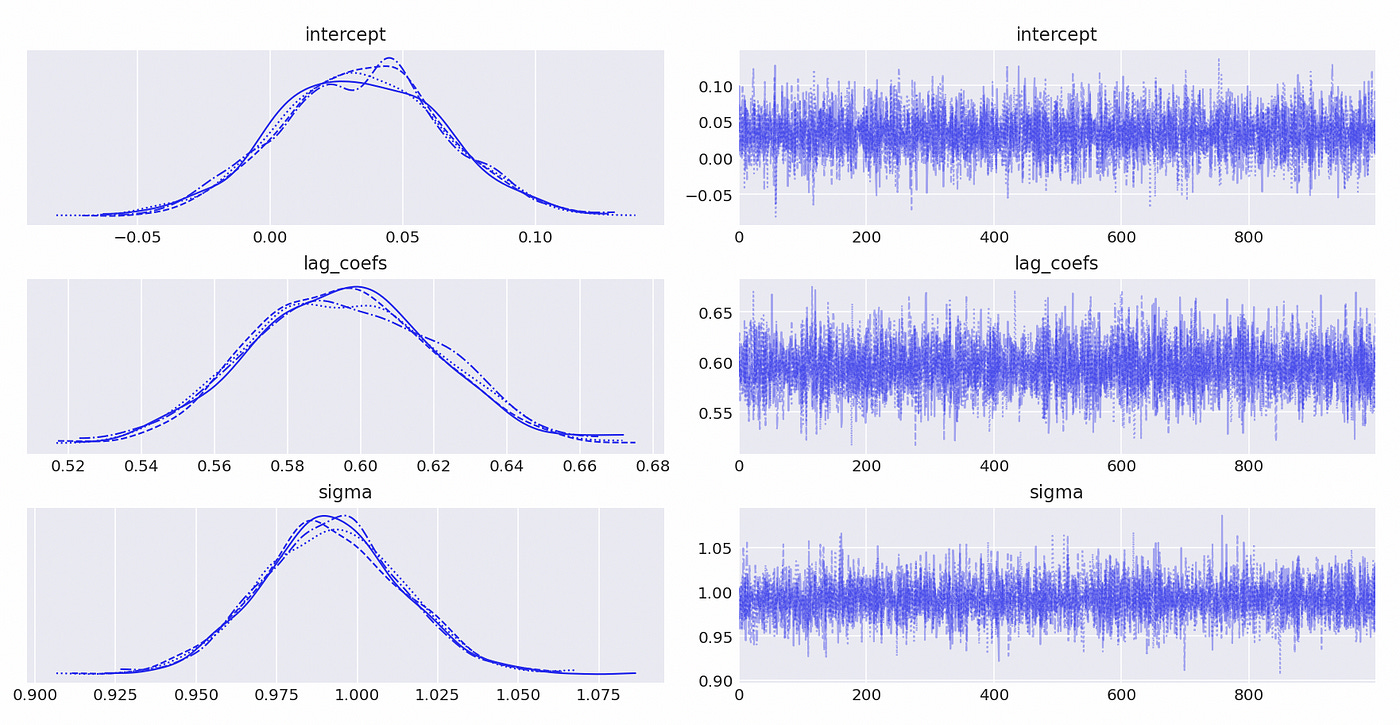
As you can see on the plot above all of the distributions have means that are close to the true parameters. We can also look at the summary statistics in the table below.
Even with uninformative (uniform) priors we were able to get very good estimates of the true parameters.
To determine if the time series is integrated we need to find the roots of characteristic polynomial, but in case of AR(1) process, reciprocal root is equal to the lag 1 coefficient. From the summary statistics and the distribution plots we can see that our estimate of lag 1 coefficient is definitely smaller than 1, which means that time series is stationary. Stationary time series are integrated of order 0 — I(0).
Now let’s try do the same with AR(2) model. Parameters of the model and roots of characteristic polynomial are show on the screenshot below.
Here let’s assume that we don’t know the order p of the model. To find it we will use the following procedure. We will fit the model for a range of lags (from 1 to 5) and select the one that has the smallest Bayesian Information Criterion (BIC). It can be easily done with a few lines of code.
On the screenshot above we see that the model with 2 lags has the smallest BIC. Therefore the order of the model is determined correctly.
Next we prepare the data and define probabilistic model. Code for doing it is provided below.
| tmpdf = pd.DataFrame.from_dict({'X':data}) | |
| tmpdf['lag_1'] = tmpdf['X'].shift() | |
| tmpdf['lag_2'] = tmpdf['X'].shift(2) | |
| tmpdf.dropna(inplace=True) | |
| X = tmpdf[['X']].values | |
| X_lags = tmpdf.drop(['X'], axis=1).values | |
| with pm.Model() as ar_model: | |
| intercept = pm.Uniform('intercept', -10, 10) | |
| lag_coefs = pm.Uniform('lag_coefs', -10, 10, shape=X_lags.shape[1]) | |
| sigma = pm.Uniform('sigma', 0, 10) | |
| mu = intercept + pm.math.sum(lag_coefs * X_lags, axis=1) | |
| obs = pm.Normal('obs', mu=mu, sigma=sigma, observed=X[:,0]) | |
| idata = pm.sample(1000) |
The model is similar to the previous one, but now we have two lag coefficients. On line 10 we define the dimensions of lag_coefs variable with shape argument. It is set to the number of columns of X_lags array, so it’ll be a general AR(p) model which will work for any number of lags, not just two.
Parameter mu defined on line 13 also changes. Basically we just implement a formula from the definition of AR(p) process with intercept:
First two terms are calculated on line 13. And the noise is defined on line 14.
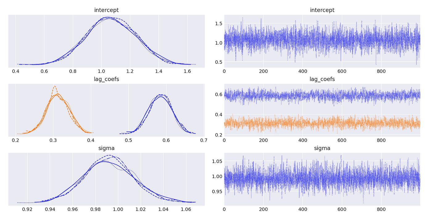
The posterior distributions above indicate that we are able to get very good estimates of true parameters. We can also confirm it with summary statistics shown below.
Recall that our end goal is to determine whether the time series is integrated. To do so we need to perform a unit root test — determine whether its largest (in absolute value) characteristic root is equal to one.
I don’t know how to calculate it inside pymc model, but we can do it from the generated sample.
| num_chains = len(idata.posterior.chain) | |
| num_draws = len(idata.posterior.draw) | |
| roots = np.zeros((num_chains,num_draws)) | |
| for c in range(num_chains): | |
| for d in range(num_draws): | |
| coefs = [1] + list(-idata.posterior['lag_coefs'][c][d].values) | |
| rts = sorted(abs(1/np.polynomial.polynomial.Polynomial(coefs).roots())) # reciprocal roots | |
| roots[c,d] = rts[-1] # largest reciprocal root in absolute value |
Each chain and each draw are processed individually. We construct characteristic polynomial from the lag coefficients of each draw, find its reciprocal roots and save the largest (in absolute value) root to a numpy array.
The resulting array can be passed to arviz plot_trace function to generate the same plots and summary statistics that we had for other parameters.
From the table above we can conclude that the largest root is less than one, which means that time series is stationary (and integrated of order 0).
We can also check some other properties of sample distribution. For example maximum value of characteristic root in a sample.
Let’s try to test a model which is integrated of order 1. Lag coefficients and characteristic roots are shown on the screenshot below. It is an AR(3) model and it has one unit root.
We use BIC to determine the order of the model.
Model with 3 lags has the lowest BIC, which is exactly what is expected.
Code for data preparation now creates 3 lags. Everything else is exactly the same.
| tmpdf = pd.DataFrame.from_dict({'X':data}) | |
| tmpdf['lag_1'] = tmpdf['X'].shift() | |
| tmpdf['lag_2'] = tmpdf['X'].shift(2) | |
| tmpdf['lag_3'] = tmpdf['X'].shift(3) | |
| tmpdf.dropna(inplace=True) | |
| X = tmpdf[['X']].values | |
| X_lags = tmpdf.drop(['X'], axis=1).values | |
| with pm.Model() as ar_model: | |
| intercept = pm.Uniform('intercept', -10, 10) | |
| lag_coefs = pm.Uniform('lag_coefs', -10, 10, shape=X_lags.shape[1]) | |
| sigma = pm.Uniform('sigma', 0, 10) | |
| mu = intercept + pm.math.sum(lag_coefs * X_lags, axis=1) | |
| obs = pm.Normal('obs', mu=mu, sigma=sigma, observed=X[:,0]) | |
| idata = pm.sample(1000) |
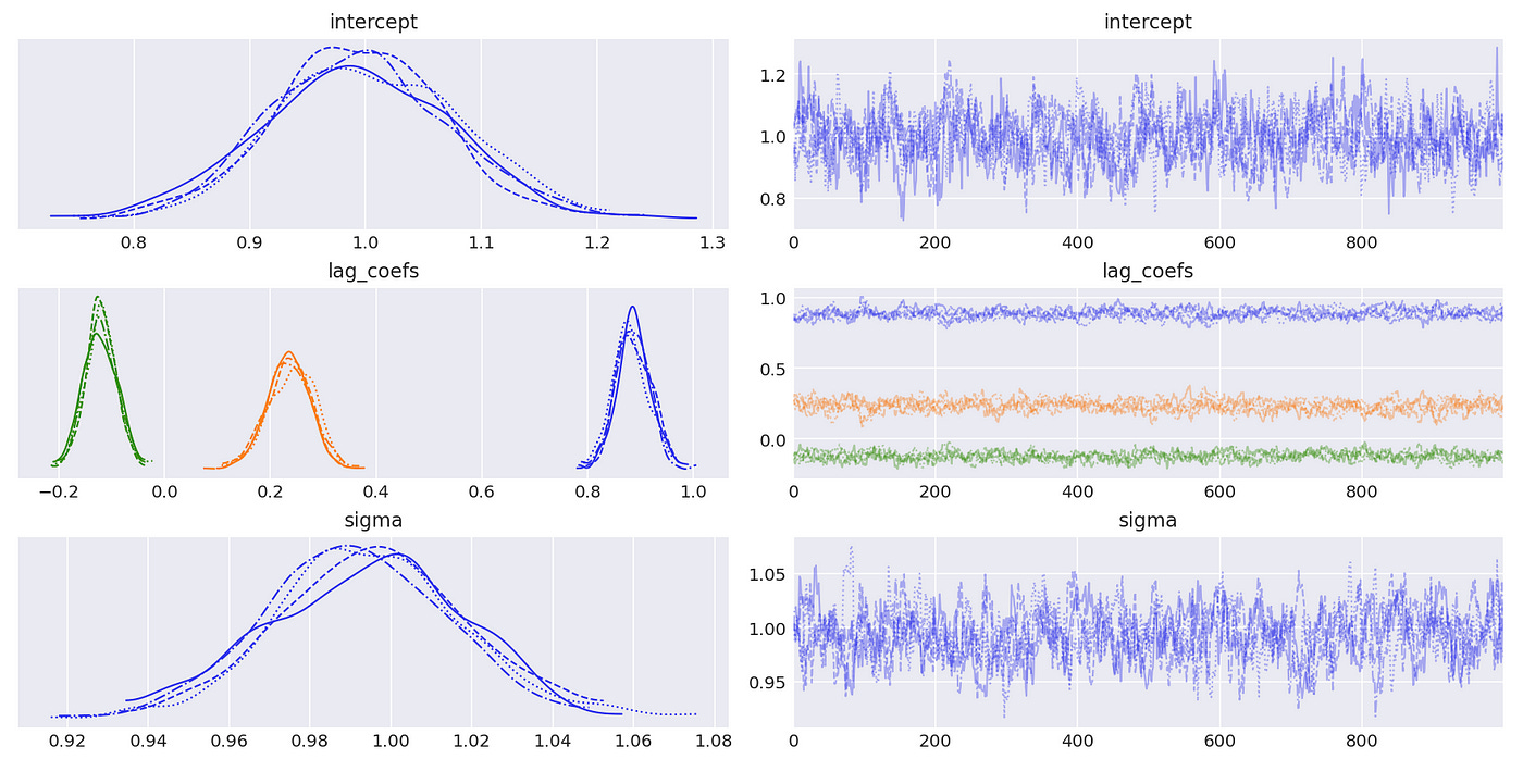
Results are presented below. And again we see that our estimates are pretty close to the true values.
Trace plot and summary statistics for largest characteristic root are shown below. We can be very confident that the given time series has unit root and therefore is integrated of order 1. The standard deviation of the posterior distribution is so small that I had to increase the number of decimals included in summary statistics.
Technically our model can be integrated of order 2 or 3 in case its second and third characteristic roots are also equal to unity, but I omit those tests for simplicity.
Now we are ready to talk about cointegrated time series. Simply put two time series are cointegrated if each of them is integrated of order 1 and there exists a linear combination of them that is stationary. This happens when the variables have the same stochastic component which can be canceled when they are combined together.
Although it is possible to talk about cointegration of two separate time series, I will skip that part and describe cointegration in multivariate vector autoregression (VAR) models. In this form it can be easily generalized to include more than two cointegrating components.
VAR model is basically a multivariate version of AR model. It can be defined as follows (for simplicity I’m going to omit deterministic terms).
The formula above defines VAR model for an n-dimensional vector x with plags. This notation is easy to understand, but to test VAR model for cointegration we need to define the model in a different way. Any VAR(p) model can be expressed as VAR(1) model. The matrix of coefficients of such representation is called companion form matrix.
There is a function in statsmodels library for constructing a companion form matrix from lag coefficient matrices B, so we don’t need to know do it ourselves. If you want to learn more theory about companion form matrix, I recommend the following resource: https://kevinkotze.github.io/ts-7-var/(part 1.2).
Analysis of VAR models is based on eigenvalues of companion form matrix. They play a similar role to the characteristic roots in univariate AR models.
First we create a function to generate a sample from VAR model with given parameters and calculate the eigenvalues of companion form matrix. Code for it is shown below.
| from statsmodels.tsa.statespace.tools import companion_matrix | |
| def generate_var(intercept, lag_coefs, eps, size=1000, return_evals=False): | |
| ''' | |
| Generate a sample from d-dimensional VAR(p) process with given parameters | |
| Order p is equal to the number of lag coefficients | |
| Args: | |
| intercept (numpy.ndarray): value of intercept with shape (p,) | |
| lag_coef (numpy.ndarray): values of lag coefficients with shape (p,d,d) | |
| eps (numpy.ndarray): standard deviation of random noise terms with shape (p,) | |
| size (int): length of sample to generate | |
| return_evals (boolean): whether to return the eigenvalues of companion matrix | |
| Returns: | |
| numpy.ndarray: generated sample (size,) | |
| list: eigenvalues of companions matrix (absolute values) | |
| ''' | |
| num_vars = lag_coefs.shape[1] | |
| lags = lag_coefs.shape[0] | |
| warmup = lags+10 | |
| x = np.zeros([warmup+size, num_vars]) | |
| x[:lags+1] = intercept | |
| for i in range(lags+1, len(x)): | |
| # prepare array of lagged variables | |
| lagged_vals = x[i-1:i-1-lags:-1] | |
| # calculate current value | |
| cs = {} | |
| for d in range(num_vars): | |
| cs[d] = intercept[d] + (lag_coefs[:,d,:]*lagged_vals).sum() + eps[d]*np.random.randn() | |
| x[i] = np.hstack([cs[d] for d in range(num_vars)]) | |
| x = x[warmup:] | |
| if return_evals: | |
| # construct companion matrix | |
| cm = companion_matrix([1] + [lag_coefs[i] for i in range(lags)]) | |
| # calculate eigenvalues and their absolute value | |
| evals = np.linalg.eig(cm)[0] | |
| evals_abs = np.abs(evals) | |
| return x, evals_abs | |
| else: | |
| return x |
To generate a sample we just implement the formula for VAR model provided above. Then on lines 24–30 we construct a companion form matrix and calculate the absolute value of its eigenvalues.
First let’s try to analyse a simple 2-dimensional VAR(1) model defined below.
There are no dependencies between the two dimensions (because the elements on counter diagonal of lag coefficient matrix are equal to zero), so each dimension is just an independent time series following AR(1) model.
Code for generating and plotting a sample from that model is shown below.
| intercept_true = np.array([1,1]) | |
| lag_coefs_true = np.array([[[0.6,0], [0,0.3]]]) | |
| sigma_true = np.array([1,1]) | |
| np.random.seed(5) | |
| data, evals = generate_var(intercept_true, lag_coefs_true, sigma_true, return_evals=True) | |
| plt.figure(figsize=(12,4)) | |
| plt.plot(data[:200,0], label='$x_1$') # plot first 200 datapoints | |
| plt.plot(data[:200,1], label='$x_2$') | |
| plt.xlabel('t') | |
| plt.ylabel('$x_t$') | |
| plt.legend() |
Absolute values of the eigenvalues are less than 1, which means that the model is covariance-stationary. We can see on the plot below that both dimensions look stationary.
Now let’s try to estimate parameters of the model using Bayesian methods. It took me some time to figure out how to define a VAR model in pymc. This article was very helpful: https://www.pymc-labs.io/blog-posts/bayesian-vector-autoregression/.
| # prepare data | |
| tmpdf = pd.DataFrame.from_dict({'x1':data[:,0], 'x2':data[:,1]}) | |
| tmpdf['x1_lag1'] = tmpdf['x1'].shift(1) | |
| tmpdf['x2_lag1'] = tmpdf['x2'].shift(1) | |
| tmpdf.dropna(inplace=True) | |
| X = tmpdf[['x1','x2']].values | |
| X_lags = tmpdf.drop(['x1','x2'], axis=1).values | |
| # define model | |
| coords = { | |
| 'lags': range(1,2), | |
| 'vars': ('x1','x2'), | |
| 'cross_vars': ('x1','x2'), | |
| 'time': range(len(X)) | |
| } | |
| with pm.Model(coords=coords) as model: | |
| intercept = pm.Uniform('intercept', -10, 10, dims=('vars')) | |
| lag_coefs = pm.Uniform('lag_coefs', -10, 10, dims=('lags','vars','cross_vars')) | |
| sigma = pm.Uniform('sigma', 0, 10, dims=('vars')) | |
| mu0 = intercept[0] + pm.math.sum(pm.math.flatten(lag_coefs[:,0,:]) * X_lags, axis=1) | |
| mu1 = intercept[1] + pm.math.sum(pm.math.flatten(lag_coefs[:,1,:]) * X_lags, axis=1) | |
| mu = pm.math.stack([mu0,mu1], axis=1) | |
| obs = pm.Normal('obs', mu=mu, sigma=sigma, observed=X, dims=('time','vars')) | |
| idata = pm.sample(1000) |
First we prepare the data. Assume that we know that the model is of lag 1. This will usually be the case for real data that we are interested in (stock prices). Data preparation step is similar to what we did before. We just have two variables (dimensions) instead of one.
The model above works for a general case of VAR(p) model with 2 dimensions. First we define the dimensions of the model in a dictionary (lines 11–16). The prior distributions of each parameter are the same as before — uniform.
For a multidimensional model we also need to define dimensions of each parameter. We have the same number of intercepts as the number of variables, so it has dimensions equal to vars (two dimensions named x1 and x2 in this case). The same is true for sigma parameter (standard deviations of random noise parameter epsilon). Dimensions of the lag coefficients follow the same notation as I used in the definition of VAR(p) model above. Let me post it here as a reminder.
Lag coefficients have the following dimensions:
Lags — corresponds to the index of matrix B (and the first subscript of matrix element beta).
Vars — corresponds to the second subscript of matrix element beta
Cross_vars — corresponds to the third subscript of matrix element beta
Our observed sample has two dimensions — number of variables in vector Xand time. Each element is calculated according to the definition of the model (lines 23–25) and in the end we have vector mu that has the same dimensions as our sample X.
On line 27 we say that each element is normally distributed with standard deviation equal to sigma.
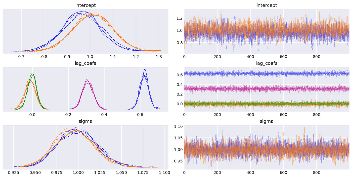
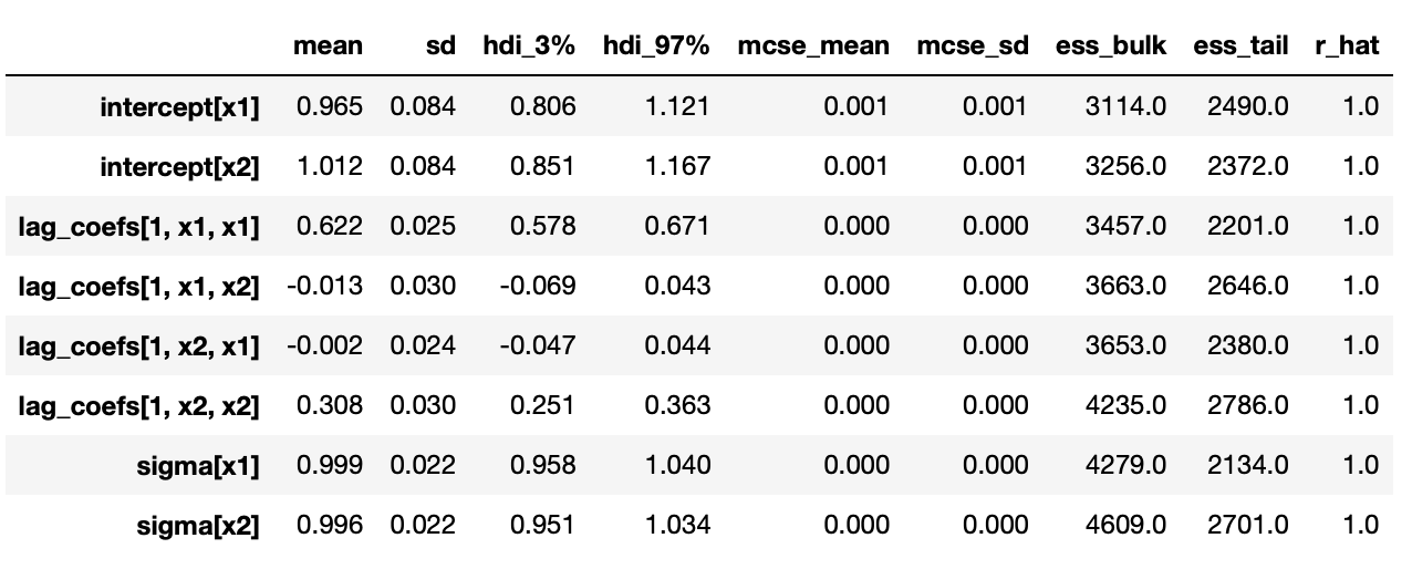
Trace plots and summary statistics are shown below.
Now let’s generate a sample with cointegrated variables and try to analyse it using Bayesian methods. The model we are going to use is defined as follows.
The third component of vector x is a pure random walk, which doesn’t depend on other two components. First two components has this same random walk in common (common stochastic trend). For the analysis of cointegration we don’t need to know what this stochastic trend is, so I will exclude it from the model and test only the first two components.
First we generate a sample from the model as shown on the screenshot below. We also confirm that the biggest eigenvalue of the companion form matrix is equal to one.
Now let’s try using traditional statistical tests for integration and cointegration.
First we use Augmented Dickey-Fuller (ADF) test on individual components. First two lines show that we can’t reject the null hypothesis of unit root (non-stationarity). On lines 3–4 we apply the same test to the first difference of each individual component. Here the null hypothesis is rejected and we can conclude that the first differences are stationary. Therefore both components are integrated of order 1.
Then we apply Engle-Granger cointegration test.
The p-value is small, therefore the null hypothesis of no-cointegration is rejected.
Now let’s try to do the same using Bayesian methods. I’ve already shown how to perform integration tests. Here I just present the results.
We can see above that the largest (in absolute value) reciprocal characteristic root is equal to one, so the time series in the first component are integrated of order one. The same is true about the second component, as shown below.
We confirmed that individual components of the vector are integrated of order one. Now to test for cointegration we need to test whether the largest eigenvalue of the companion form matrix is equal to unity. Code for doing it is shown below.
| # prepare data | |
| tmpdf = pd.DataFrame.from_dict({'x1':data[:,0], 'x2':data[:,1]}) | |
| tmpdf['x1_lag1'] = tmpdf['x1'].shift(1) | |
| tmpdf['x2_lag1'] = tmpdf['x2'].shift(1) | |
| tmpdf.dropna(inplace=True) | |
| # fit VAR(1) model | |
| X = tmpdf[['x1','x2']].values | |
| X_lags = tmpdf.drop(['x1','x2'], axis=1).values | |
| coords = { | |
| 'lags': range(1,2), | |
| 'vars': ('x1','x2'), | |
| 'cross_vars': ('x1','x2'), | |
| 'time': range(len(X)) | |
| } | |
| with pm.Model(coords=coords) as model: | |
| intercept = pm.Uniform('intercept', -10, 10, dims=('vars')) | |
| lag_coefs = pm.Uniform('lag_coefs', -10, 10, dims=('lags','vars','cross_vars')) | |
| sigma = pm.Uniform('sigma', 0, 10, dims=('vars')) | |
| mu0 = intercept[0] + pm.math.sum(pm.math.flatten(lag_coefs[:,0,:]) * X_lags, axis=1) | |
| mu1 = intercept[1] + pm.math.sum(pm.math.flatten(lag_coefs[:,1,:]) * X_lags, axis=1) | |
| mu = pm.math.stack([mu0,mu1], axis=1) | |
| obs = pm.Normal('obs', mu=mu, sigma=sigma, observed=X, dims=('time','vars')) | |
| idata = pm.sample(1000) | |
| # find the distribution of the largest eigenvalue | |
| num_chains = len(idata.posterior.chain) | |
| num_draws = len(idata.posterior.draw) | |
| evals = np.zeros((num_chains,num_draws)) # largest eigenvalue | |
| for c in range(num_chains): | |
| for d in range(num_draws): | |
| cm = companion_matrix([1] + [idata.posterior['lag_coefs'][c][d][0].values]) | |
| max_eval = sorted(abs(np.linalg.eig(cm)[0]))[-1] | |
| evals[c,d] = max_eval |
I already explained how we define VAR(1) model in pymc. The only new part is finding the distribution of the largest eigenvalue. It is very similar to how we found the distribution of characteristic roots. And again, I don’t know how to do it inside the model, so we just process each chain and each draw separately. For each draw, we construct a companion matrix, calculate its eigenvalues and save the largest eigenvalue in the numpy array.
That array is then passed to arviz to generate posterior plots and summary statistics. Results are shown below.
We can be pretty sure that the largest eigenvalue is very close to 1, so we can conclude that the time series are indeed cointegrated.
Unlike traditional statistical tests, with Bayesian methods we are able to get a whole posterior distribution of the parameter of interest. This gives use a lot more flexibility in what types of inference we can make. But this article is already too long and I think we can stop here. In the next article I will try to implement more modern version of Bayesian cointegration analysis and backtest a trading strategy based on it.
Jupyter notebook with source code is available here.
If you have any questions, suggestions or corrections please post them in the comments. Thanks for reading.
References
[2] Bayesian Vector Autoregression in PyMC
[3] Vector autoregression models
[4] Cointegration


