Granger causality test in pairs trading
Improving pairs trading strategies with causal analysis.

Many traditional pairs trading strategies use cointegration tests for pair selection. If a pair of stocks is found to be cointegrated then this pair is accepted for trading. In this article I will check if using Granger causality test in pair selection process can improve the performance of such strategies. Idea for this article comes from the paper ‘Illuminating the Profitability of Pairs Trading: A Test of the Relative Pricing Efficiency of Markets for Water Utility Stocks’ (Gutierrez and Tse, 2011).
Granger causality test is a statistical test that allows us to check if one time series is useful in predicting another. Here is a nice summary of intuition behind this test from wikipedia:
We say that a variable X that evolves over time Granger-causes another evolving variable Y if predictions of the value of Y based on its own past values and on the past values of X are better than predictions of Y based only on Y’s own past values.
If variable X Granger-causes variable Y, then X is called Granger-leader and Y is called Granger-follower.
Assume we know which stock is Granger-leader and which is Granger-follower. How can it help in pairs trading? First of all, we now know which stock should be a dependent variable and which stock should be an independent variable in the OLS model for constructing a spread (Granger-leader — independent, Granger-follower-dependent). It was unclear when we used just cointegration test. Second thing we can do is to open positions only in Granger-follower, assuming that most of the profit will come from it following a movement of Granger-leader.
To test this idea I will first implement a simple cointegration-based trading strategy to use as a baseline. Then I will modify it to include Granger causality tests and see how it affects the performance.
I am going to use the same stock universe as in my previous article: 100 stocks from VBR Small-Cap ETF. I will use a 3-year period from 2010–01–01to 2012–12–31. First two years will be used as a formation period for pair selection and last year will be used as a trading period.
We start with loading and preparing the data. Code for doing it is provided below.
| stocks = ['TRN', 'BDN', 'CMC', 'NYT', 'LEG', 'VNO', 'HLX', 'ORI', 'HP', 'EQC', 'MTOR', | |
| 'DKS', 'SEE', 'EAT', 'AGCO', 'AIV', 'WSM', 'BIG', 'HFC', 'AN', 'ENDP', 'OI', | |
| 'FFIV', 'AXL', 'VSH', 'NCR', 'MDRX', 'UIS', 'CRUS', 'FLR', 'MUR', 'ATI', 'PBI', | |
| 'PWR', 'TEX', 'RRC', 'FL', 'NVAX', 'LPX', 'CMA', 'AMKR', 'RMBS', 'MFA', 'ZION', | |
| 'HOG', 'UNM', 'IVZ', 'NWL', 'GME', 'JWN', 'NUAN', 'ANF', 'FHN', 'JBL', 'URBN', | |
| 'PBCT', 'HRB', 'LNC', 'RDN', 'TGNA', 'NYCB', 'WEN', 'CNX', 'STLD', 'TOL', 'BBBY', | |
| 'APA', 'MAT', 'BPOP', 'KBH', 'PTEN', 'SANM', 'DVN', 'MOS', 'OVV', 'TPR', 'CLF', | |
| 'AEO', 'KSS', 'SWN', 'MTG', 'GT', 'NOV', 'CDE', 'IPG', 'JBLU', 'THC', 'ODP', | |
| 'RIG', 'SNV', 'M', 'ON', 'GPS', 'X', 'MRO', 'XRX', 'JNPR', 'CAR', 'RAD', 'SLM'] | |
| start = '2010-01-01' | |
| end = '2012-12-31' | |
| trn = yf.download('TRN', start, end) | |
| prices = pd.DataFrame(index=trn.index, columns=stocks) | |
| prices['TRN'] = trn['Adj Close'] | |
| for s in stocks[1:]: | |
| pdf = yf.download(s, start, end) | |
| prices[s] = pdf['Adj Close'] | |
| log_prices = np.log(prices) | |
| returns = prices.pct_change().dropna() | |
| log_returns = log_prices.diff().dropna() | |
| form_start = '2010-01-01' | |
| form_end = '2011-12-31' | |
| trade_start = '2012-01-01' | |
| trade_end = '2012-12-31' | |
| log_prices_form = log_prices.loc[form_start:form_end] | |
| log_prices_trade = log_prices.loc[trade_start:trade_end] | |
| log_returns_form = log_returns.loc[form_start:form_end] | |
| log_returns_trade = log_returns.loc[trade_start:trade_end] | |
| returns_form = returns.loc[form_start:form_end] | |
| returns_trade = returns.loc[trade_start:trade_end] |
Second step is pair selection. I will select pairs based on Cointegrated Augmented Dickey-Fuller (CADF) test. I test log price series of each pair for cointegration and select only those which have CADF-test pvalue less than 0.01. Moreover I select only pairs with different stocks: if a given stock is already used in some selected pair, I don’t accept any other pairs with it.
| selected_pairs = [] | |
| selected_stocks = [] | |
| for s1 in stocks: | |
| for s2 in stocks: | |
| if (s1!=s2) and (s1 not in selected_stocks) and (s2 not in selected_stocks): | |
| if (coint(log_prices_form[s1], log_prices_form[s2])[1] < 0.01): | |
| selected_stocks.append(s1) | |
| selected_stocks.append(s2) | |
| selected_pairs.append(f'{s1}-{s2}') |
Assume that we have two cointegrated stocks X and Y. Then we can represent (log) price of stock X as follows:
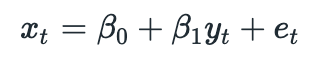
The last term is called disturbance term (or spread). The fact that two time series are cointegrated implies that spread must be stationary (it has constant mean and constant variance). This means that any deviations from the mean are temporary. From the equation above we have:
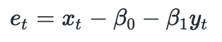
Coefficients beta_0 and beta_1 are calculated by fitting an Ordinary Least Squares (OLS) model to historical data (from formation period). Spread mean and standard deviation are calculated from the same data.
The rules for opening positions are as follows:
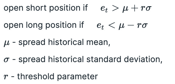
Here short position in spread means selling stock X and buying stock Y. Long position means buying stock X and selling stock Y. Positions are closed when the spread returns back to its mean.
In the paper mentioned above authors test several values for threshold parameter r — 0.25, 0.5 and 0.75. I am going to test only one value r=0.75. Code for backtesting a baseline algorithm is provided below.
| r = 0.75 # standard deviation threshold | |
| positions_short = pd.DataFrame(index=returns_trade.index, columns=selected_stocks) | |
| positions_long = pd.DataFrame(index=returns_trade.index, columns=selected_stocks) | |
| for pair in selected_pairs: | |
| s1,s2 = parse_pair(pair) | |
| # calculate parameters using historical data | |
| model = sm.OLS(log_prices_form[s1], sm.add_constant(log_prices_form[s2])) | |
| res = model.fit() | |
| mu = res.resid.mean() # spread historical mean | |
| sigma = res.resid.std() # spread historical sd | |
| # calculate spread | |
| spread = log_prices_trade[s1] - res.predict(sm.add_constant(log_prices_trade[s2])) | |
| # calculate positions | |
| positions_short.loc[spread > mu+r*sigma, [s1,s2]] = [-1,1] | |
| positions_short.loc[spread < mu, [s1,s2]] = [0,0] | |
| positions_long.loc[spread < mu-r*sigma, [s1,s2]] = [1,-1] | |
| positions_long.loc[spread > mu, [s1,s2]] = [0,0] | |
| positions_short.fillna(method='ffill', inplace=True) | |
| positions_short.fillna(0, inplace=True) | |
| positions_long.fillna(method='ffill', inplace=True) | |
| positions_long.fillna(0, inplace=True) | |
| positions = positions_long + positions_short | |
| # calculate returns | |
| ret = (positions.shift() * returns_trade[selected_stocks]).sum(axis=1)/len(selected_pairs) | |
| cumret = np.nancumprod(ret + 1) |
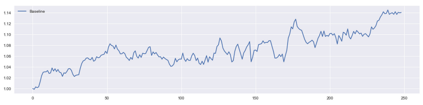
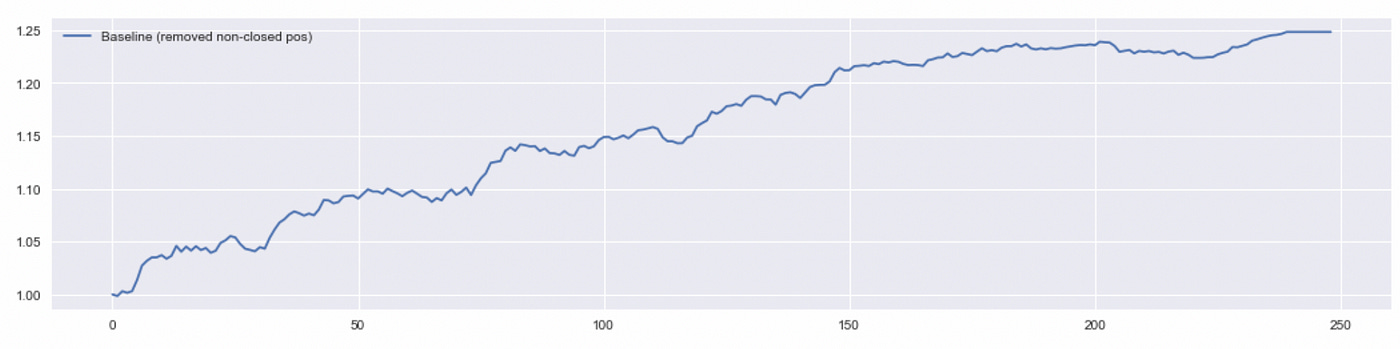
We get a total return of about 14% which is not bad.
Another thing I will try to do is to remove all positions that are not closed by the end of the trading period. I am not sure that it is a correct way to perform a backtest (because it introduces a look-ahead bias), but it is done in the paper, so I’ll do it too. We just edit positions dataframe using the code below and recalculate the returns.
| # remove positions that are not closed by the end of trading period | |
| for s in positions.columns: | |
| for t in positions.index[::-1]: | |
| if positions.loc[t,s]==0: | |
| break | |
| else: | |
| positions.loc[t,s]=0 |
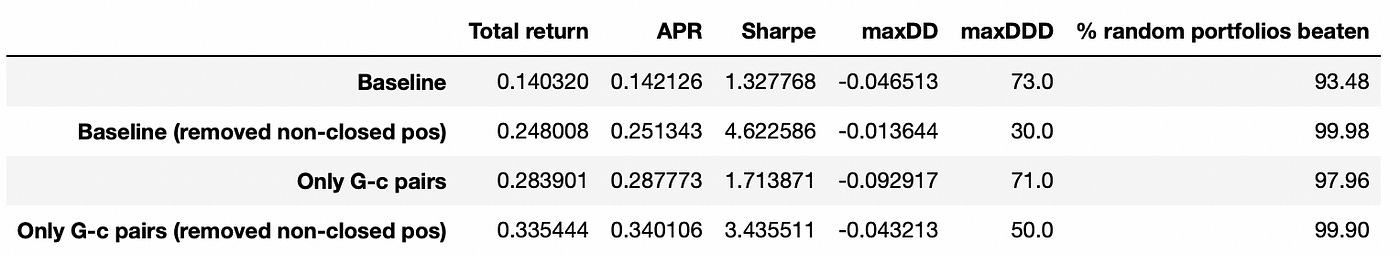
As we see above, removing non-closed positions nearly doubles total return of the strategy. Let’s look at performance metrics of these two algorithms. The last column in the table below is calculated using a bootstrap method. It is described in detail in my previous post.
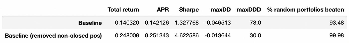
The results look quite good, but keep in mind that I didn't include transaction costs in my backtests. Let’s see if performance can be improved with Granger causality test.
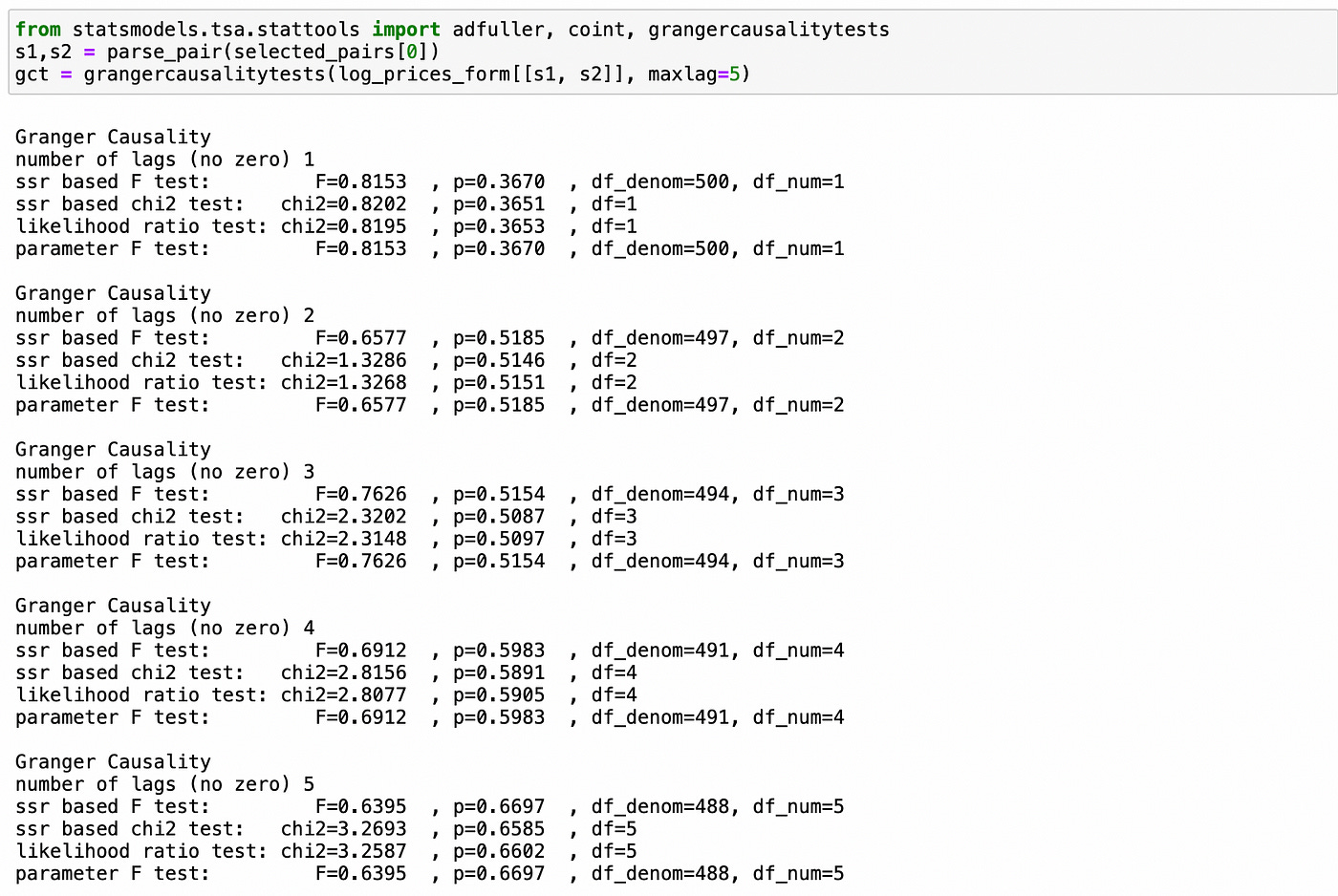
Granger causality test is implemented in statsmodels library. Let’s see how it works. Below I perform the test for one of the selected pairs. The order of columns in the tested dataframe does matter: first column is assumed to be Granger-follower and second column is assumed to be Granger-leader. I set parameter maxlag=5 so that we can select only those pairs which converge back to the equilibrium fast enough. Pvalues indicate the probability that a given lag of time series in the second column does NOT influence the values in the first column. In this particular case we see that we can’t reject the null hypothesis of absence of Granger causality. Four different tests are performed for each lag, but they all give pvalues that are very close to each other.
Now I will try to apply Granger causality test to pair selection process. I will process each of the cointegrated pairs (selected above) and select only those pairs which have pvalue less than 0.01 for at least one of the lags. Note that for each pair we need to perform two tests (switching Granger-leader and Granger-follower).
| maxlag=5 | |
| selected_pairs_gc = [] | |
| selected_stocks_gc = [] | |
| for pair in selected_pairs: | |
| s1,s2 = parse_pair(pair) | |
| gct12 = grangercausalitytests(log_prices_form[[s1,s2]], maxlag=maxlag) | |
| pvals12 = [gct12[x][0]['ssr_ftest'][1] for x in range(1,maxlag+1)] | |
| pvals12 = np.array(pvals12) | |
| if len(pvals12[pvals12<0.01])>0: | |
| selected_pairs_gc.append(f'{s1}-{s2}') | |
| selected_stocks_gc.append(s1) | |
| selected_stocks_gc.append(s2) | |
| else: # switch Granger-leader and Granger-follower | |
| gct21 = grangercausalitytests(log_prices_form[[s2,s1]], maxlag=maxlag) | |
| pvals21 = [gct21[x][0]['ssr_ftest'][1] for x in range(1,maxlag+1)] | |
| pvals21 = np.array(pvals21) | |
| if len(pvals21[pvals21<0.01])>0: | |
| selected_pairs_gc.append(f'{s2}-{s1}') | |
| selected_stocks_gc.append(s2) | |
| selected_stocks_gc.append(s1) |
After running the code above we get only 10 pairs (out of 21 we got after performing CADF-test). Now I’m going to backtest exactly the same strategy as before, but using only 10 selected pairs.
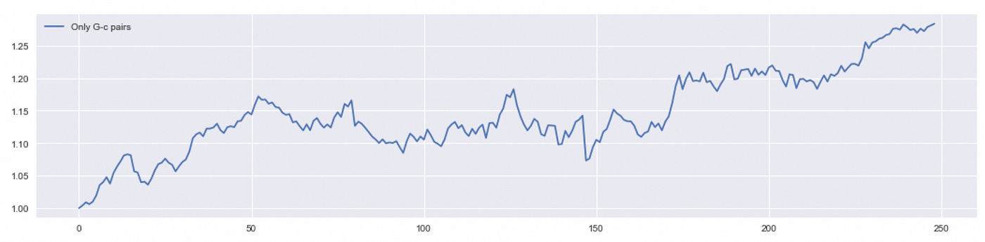
Total return is about 28%, which is twice as much as return of the baseline strategy. I will also try removing positions that are not closed before the end of the trading period. Performance metrics of the algorithms tested so far are provided below.
We see that using only pairs that pass Granger causality test significantly improves the performance of this strategy. We can try to improve it even more. It is said in the paper that most of the profit comes from trading in Granger-follower. Let’s try to test it.
| r = 0.75 # standard deviation threshold | |
| positions_short = pd.DataFrame(index=returns_trade.index, columns=selected_stocks_gc) | |
| positions_long = pd.DataFrame(index=returns_trade.index, columns=selected_stocks_gc) | |
| for pair in selected_pairs_gc: | |
| s1,s2 = parse_pair(pair) | |
| # calculate parameters using historical data | |
| model = sm.OLS(log_prices_form[s1], sm.add_constant(log_prices_form[s2])) | |
| res = model.fit() | |
| mu = res.resid.mean() # spread historical mean | |
| sigma = res.resid.std() # spread historical sd | |
| # calculate spread | |
| spread = log_prices_trade[s1] - res.predict(sm.add_constant(log_prices_trade[s2])) | |
| # calculate positions | |
| positions_short.loc[spread > mu+r*sigma, [s1,s2]] = [-1,0] | |
| positions_short.loc[spread < mu, [s1,s2]] = [0,0] | |
| positions_long.loc[spread < mu-r*sigma, [s1,s2]] = [1,0] | |
| positions_long.loc[spread > mu, [s1,s2]] = [0,0] | |
| positions_short.fillna(method='ffill', inplace=True) | |
| positions_short.fillna(0, inplace=True) | |
| positions_long.fillna(method='ffill', inplace=True) | |
| positions_long.fillna(0, inplace=True) | |
| positions = positions_long + positions_short | |
| ret = (positions.shift() * returns_trade[selected_stocks_gc]).sum(axis=1)/len(selected_pairs_gc) | |
| cumret = np.nancumprod(ret + 1) |
In the code above you can see that now we trade only in the first stock of the pair, which is a Granger follower (lines 16 and 18).
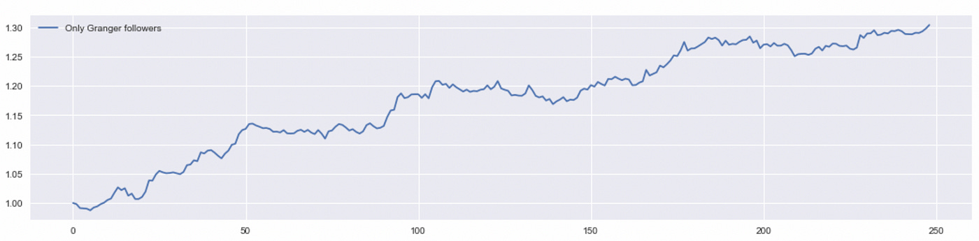
We don’t get a significant improvement in performance, but it is still an improvement. It means that removing positions in Granger-leaders allowed us to cut some losses. Let’s compare performance metrics of all of the tested strategies.
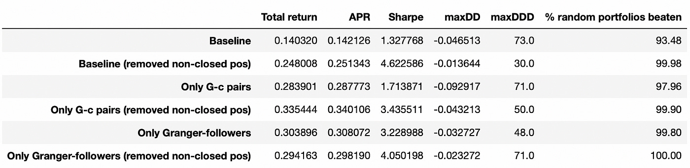
We can see that applying Granger causality test to pair selection can provide a significant increase in performance of the strategy. Baseline strategy with removed non-closed positions has the biggest Sharpe ratio, but I want to emphasize again that such backtests contain a look-ahead bias, so it is better to compare only strategies without removed positions.
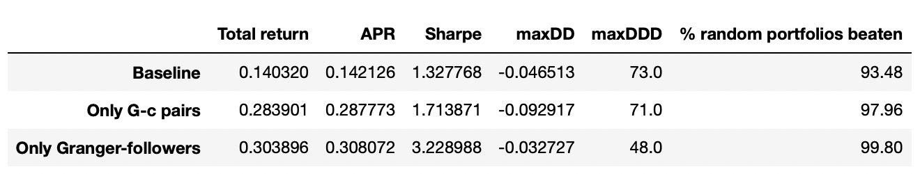
Strategy trading only in Granger-followers performs better than two other strategies in terms of any metric calculated above. With transaction costs, its performance relative to other strategies would be even better (because we trade only in one stock per pair instead of two). We can also see that all of the strategies perform better than random trading using bootstrap method (last column).
Overall I think that Granger causality test can be a useful instrument in pairs trading. It would be interesting to test it in application to other pairs trading strategies.
Jupyter notebook with source code is available here.
If you have any questions, suggestions or corrections please post them in the comments. Thanks for reading.
References
[2] Statistical arbitrage pairs trading strategies: Review and outlook (Krauss, 2015)