Sometimes in finance it is necessary to model marginal returns of a given asset. Marginal in this case means that there are no serial correlations between returns in different time periods (returns are independent and identically distributed). A couple of examples:
We might believe that returns of a certain asset do not have any serial correlations, in that case we can increase the statistical significance of our backtests by running many simulations to assess strategy performance (each time drawing asset returns from the modeled distribution).
Even if we find that returns are serially correlated, we might want to test a scenario in which the correlations we found are spurious (again run many simulations and look at maximum drawdown).
In this article I will demonstrate several techniques which can be used for modeling marginal returns.
The simplest approach is just to sample returns from historical data, but in this case the sample size would be too small, especially for longer time periods. Another approach is to model probability distribution of the returns. We can then get simulated returns just by sampling from that distribution. Now the problem is to determine which distribution we should use. There are several ways to do it:
Looking at the data and trying to guess which one of well-known parametric distributions (or time series models) it follows, then applying goodness-of-fit tests to determine if our guess was correct.
Using Pearson system, which takes sample mean, variance, skewness and kurtosis as an input and models the data as one of the seven probability distribution families.
Using quantile-parameterized distribution which is parameterized by data.
Using metalog distribution which seems to be the most flexible of all techniques.
I was not able to find an implementation of quantile-parameterized distributions in Python, so I will only demonstrate three other methods. Let’s get started.
I will use daily returns of SPY ETF from 1993 to 2022 as my sample (7318 observations in total). Let’s have a look at the data. First we will look at some summary statistics.
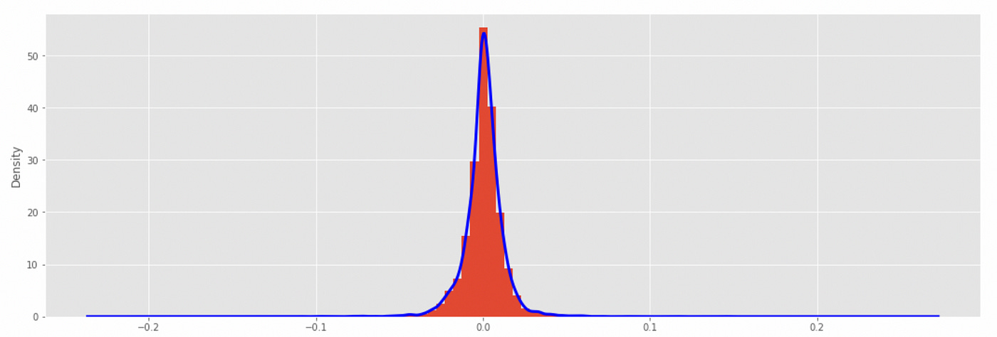
The mean return is very close to zero and the range of returns is approximately from -0.11 to 0.15. Now let’s look at the histogram and empirical probability density function.
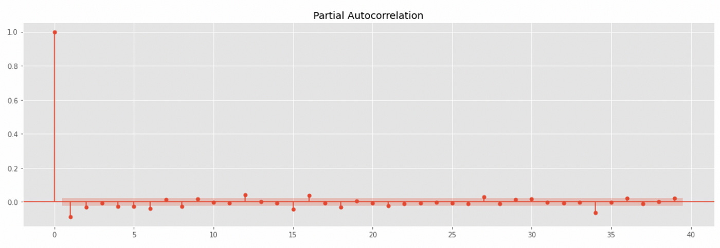
At first glance the distribution looks symmetric and kind of similar to Gaussian distribution. Next we take a look at the autocorrelation and partial autocorrelation plots. It will help us understand if there are any serial correlations in the data.
Even though autocorrelation coefficients for some lags exceed confidence interval, they are still very low (less than 0.1 in absolute value), so the assumption that there are no serial correlations might not be wrong.
Now I will demonstrate several techniques to model marginal returns. I will assess the performance of each technique using QQ-plots and Kolmogorov-Smirnov goodness-of-fit test.
Parametric distributions
First I will try fitting several well-known probability distributions: normal distribution, lognormal distribution, and Student’s t-distribution.
| from scipy import stats | |
| import statsmodels.api as sm | |
| from scipy.stats import kstest | |
| x = np.linspace(-0.15, 0.15, 1000) | |
| plt.figure(figsize=(18,6)) | |
| plt.subplot(121) | |
| loc,scale = stats.norm.fit(spy_ret) | |
| plt.plot(x, stats.norm.pdf(x, loc=loc, scale=scale), label='Normal') | |
| spy_ret.plot(kind='kde', label='Empirical') | |
| plt.legend() | |
| plt.subplot(122) | |
| _ = sm.qqplot(spy_ret, stats.norm(loc=loc, scale=scale), line='45', ax=plt.gca()) | |
| # Kolmogorov-Smirnov test | |
| kstest(spy_ret, stats.norm.rvs(size=len(spy_ret), loc=loc, scale=scale), N=5000) |
The code above is for normal distribution. First we fit the given distribution on our data using SciPy fit function. It provides us with parameters that define a given distribution. Then I create two plots: a plot of empirical probability density function (PDF) along with model PDF and a QQ-plot to compare empirical and modeled distributions. These plots are demonstrated below.
Just by looking at the plots above we can see that normal distribution is a bad choice. The last step is to perform Kolmogorov-Smirnov goodness-of-fit test. I am drawing samples from a modeled distribution and then using 5000 samples to compare modeled and empirical distributions. Results of the test are provided below.
P-value is almost zero, which means that there is zero percent chance that two distributions are equal.
Let’s try lognormal distribution. The code I used is very similar, so I won’t post it here. Below you can see generated plots and results of Kolmogorov-Smirnov test.
The results we get here are almost identical to the previous ones, so lognormal distribution is also not a good choice.
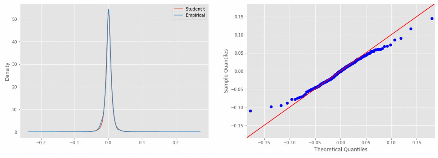
How about Student’s t-distribution?
Here we are getting very close. The plots of PDFs match each over very closely, but at QQ-plot we can see that the tails of the modeled distribution do not fit very well. Kolmogorov-Smirnov test gives a p-value of 0.12, which means that there is a 12% chance that tested samples come from the same distribution, which is not that bad. Let’s move on to other methods.
Pearson system
Pearson system allows us to model probability distribution based on several empirical moments (mean, variance, skewness and kurtosis). There are seven families of distributions that can be modeled using Pearson system and Student’s t-distribution used above is actually one of it. Unfortunately only Pearson type III distributions are implemented in SciPy, but it is a very bad fit for our data. You can see it on the plots below.
Metalog distribution
Metalog distribution is one of the newest and most flexible distribution families. It was introduced in 2016 and provides many advatages compared to other methods. You can read about it here and here. It’s implementation for Python can be found here.
When using metalog distributions we need to specify the number of terms used to describe the shape of the distribution (it can range from 2 to 30). The larger the number of terms the more flexible the shape of the distribution can be. To determine the number of terms to use I will test a range of values from 2 to 13 and select the one which gives the largest p-value in Kolmogorov-Smirnov test. Code for doing that is provided below.
| from metalog import metalog | |
| metalog_ret = metalog.fit(spy_ret.values, step_len=0.001) | |
| best_t, best_stat = None, float('Inf') | |
| for t in range(2,14): | |
| stat,pval = kstest(spy_ret, metalog.r(m=metalog_ret, n=len(spy_ret), term=t), N=5000) | |
| if stat<best_stat: | |
| best_stat = stat | |
| best_t = t | |
| print(stat,pval) | |
| print(f'Best number of terms: {best_t}') |
Running this code gives the following output:
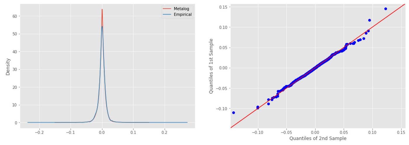
The best results is achieved with 11 terms, giving a p-value of 0.85, which means that there is an 85% chance that the samples are drawn from the same distribution (empirical and modeled distributions are the same). This is the best result achieved so far. Let’s look at the plots.
| plt.figure(figsize=(18,6)) | |
| plt.subplot(121) | |
| plt.plot(x, metalog.d(m=metalog_ret, q=x, term=11), label='Metalog') | |
| spy_ret.plot(kind='kde', label='Empirical', figsize=(18,6)) | |
| plt.legend() | |
| plt.subplot(122) | |
| _ = sm.qqplot_2samples(spy_ret, metalog.r(m=metalog_ret, n=len(spy_ret), term=11), line='45', ax=plt.gca()) |
As we can see above, PDFs of the distributions match each other very closely. QQ-plot also looks nice, but there are still some small discrepancies in the tails (which is to be expected considering that such returns are extremely rare and our sample size is not that big). Probably to be able to better model probabilities of extremely rare returns we would need to use Extreme Value Theory.
In this article I have demonstrated several methods of modeling marginal returns distributions. We have seen that out of all tested distributions only two have provided more or less acceptable results: Student’s t-distribution and metalog distribution. It seems that using metalog family of distributions is the best of all tested options.
Jupyter notebook with source code is available here.
If you have any questions, suggestions or corrections please post them in the comments. Thanks for reading.


