Pairs trading. Modeling the spread with mean-reverting Gaussian Markov chain model
State-space models in pairs trading.

This article is based on the paper ‘Pairs Trading’ by Elliot et al. (2005). The paper describes how we can model the spread as a mean-reverting Gaussian Markov chain observed in Gaussian noise and how to calibrate such model from market observations. I will implement one of the proposed algorithms for parameter estimation and backtest a simple strategy based on it.
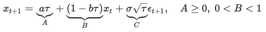
The proposed model is a state-space model which is described by two equations. The state equation is:

Note that we can rewrite it as:
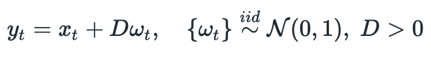
The observation equation is:
So now, if we know the parameters of the model (A,B,C,D), we can use Kalman filter to estimate the current state of the spread and try to predict the next state of the spread. I will describe how it can be used for trading later, when I implement a trading strategy. For now let’s look at the process for parameter estimation.
Parameter estimation is done using expectation maximization (EM) algorithm. In the paper authors propose two implementations of EM algorithm. I will implement Shumway and Stoffer smoother approach described in section 3.2.1. I can’t dig deep into the math of this approach because to be honest I don’t understand it very well. But I was able to implement it in Python, using the formulas provided in the paper, and it seems to work.
Basic idea is the following:
make initial guess of parameters A,B,C,D
run Kalman filter on historical prices of the spread
run backward recursion on the values we got from Kalman filter
update parameters A,B,C,D according to given formulas
The algorithm above is repeated a given number of iterations and in the end we get our estimates of parameters A,B,C,D. The code of my implementation of this algorithm is provided below. I think it is easier to understand it by looking at the code instead of mathematical formulas.
| def ss_smoother(y, init_params, num_iter=150, x_0=0, R_0=0.1): | |
| ''' | |
| run Shumway Stoffer smoother algorithm with given initial values | |
| x_0, R_0 - inital guesses for Kalman filter | |
| ''' | |
| N = len(y) | |
| A,B,C,D = [np.zeros(num_iter) for _ in range(4)] | |
| A[0],B[0],C[0],D[0] = init_params['A'], init_params['B'], init_params['C'], init_params['D'] | |
| x_N, R_N = [x_0], [R_0] # initial guesses for Kalman filter | |
| # run algorithm for num_iter iterations | |
| for i in range(1,num_iter): | |
| # run Kalman filter | |
| x_pred = np.zeros(N) | |
| R_pred = np.zeros(N) | |
| x0 = x_N[0] | |
| R0 = R_N[0] | |
| for k in range(0,N): | |
| # predict | |
| if k==0: | |
| x_hat = A[i-1] + B[i-1] * x0 | |
| R_hat = B[i-1]**2 * R0 + C[i-1]**2 | |
| else: | |
| x_hat = A[i-1] + B[i-1] * x_pred[k-1] | |
| R_hat = B[i-1]**2 * R_pred[k-1] + C[i-1]**2 | |
| # update | |
| K = R_hat / (R_hat + D[i-1]**2) | |
| x_pred[k] = x_hat + K * (y[k] - x_hat) | |
| R_pred[k] = D[i-1]**2 * K | |
| # run Shumway-Stoffer backward recursion | |
| x_N = np.zeros(N) | |
| R_N = np.zeros(N) | |
| J = np.zeros(N) | |
| x_N[-1] = x_pred[-1] | |
| R_N[-1] = R_pred[-1] | |
| for k in range(N-2,-1,-1): | |
| J[k] = B[i-1] * R_pred[k] / ((B[i-1])**2 * R_pred[k] + (C[i-1])**2) | |
| x_N[k] = x_pred[k] + J[k] * (x_N[k+1] - (A[i-1] + B[i-1] * x_pred[k])) | |
| R_N[k] = R_pred[k] + J[k]**2 * (R_N[k+1] - ((B[i-1])**2 * R_pred[k] + (C[i-1])**2)) | |
| # compute alpha | |
| alpha = np.sum(R_N[:-1] + (x_N**2)[:-1]) | |
| # beta | |
| sigma_kN = np.zeros(N) | |
| sigma_kN[-1] = B[i-1] * (1 - K) * R_pred[-1] # i'm not sure about the last term, but it seems that it works | |
| for k in range(N-2,-1,-1): | |
| sigma_kN[k] = J[k] * R_pred[k+1] + J[k+1]*J[k] * (sigma_kN[k+1] - B[i-1] * R_pred[k+1]) | |
| beta = np.sum(sigma_kN[:-1] + x_N[1:] * x_N[:-1]) | |
| # gamma, delta | |
| gamma = np.sum(x_N[1:]) | |
| delta = gamma - x_N[-1] + x_N[0] | |
| # update parameters | |
| A[i] = (alpha * gamma - delta*beta) / (N*alpha - delta**2) | |
| B[i] = (N*beta - gamma*delta) / (N*alpha - delta**2) | |
| C[i] = np.sqrt(1/(N-1) * np.sum(R_N[1:] + x_N[1:]**2 + A[i]**2 + B[i]**2 * R_N[:-1] | |
| + B[i]**2 * x_N[:-1]**2 - 2*A[i]*x_N[1:] + 2*A[i]*B[i]*x_N[:-1] | |
| - 2*B[i]*sigma_kN[:-1] - 2*B[i]*x_N[1:]*x_N[:-1])) | |
| D[i] = np.sqrt(1/N * np.sum(y**2 - 2*y*x_N + R_N + x_N**2)) | |
| return {'A':A, 'B':B, 'C':C, 'D':D} |
Now I will replicate a numerical example provided in part 4 of the paper. First we generate 100 data points according to the model with parameters: A=0.2, B=0.85, C=0.60, D=0.8. The code of data generating function is provided below.
| def generate_data(params, N=100): | |
| ''' | |
| generate observations of stochastic process with parameters A, B, C, D | |
| ''' | |
| epsilon = np.random.randn(N) | |
| w = np.random.randn(N) | |
| x = np.zeros(N) # states | |
| x[0] = 0 | |
| for k in range(1,N): | |
| x[k] = params['A'] + params['B']*x[k-1] + params['C']*epsilon[k] | |
| y = x + params['D']*w # observations | |
| return y |
After that we run EM algorithm for 150 iterations with the following initial parameters: A=1.2, B=0.5, C=0.30, D=0.7. Below you can see the results.
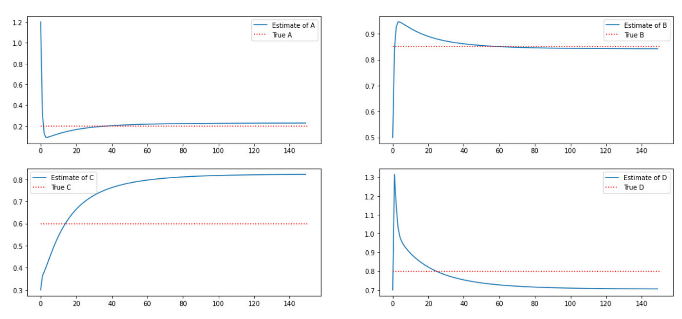
Results look very similar to the plots provided in the paper. Of course we can’t achieve perfect replication due to stochastic nature of the process. I also tried running the same example using 1000 data points and was able to get estimates which are very close to true values:
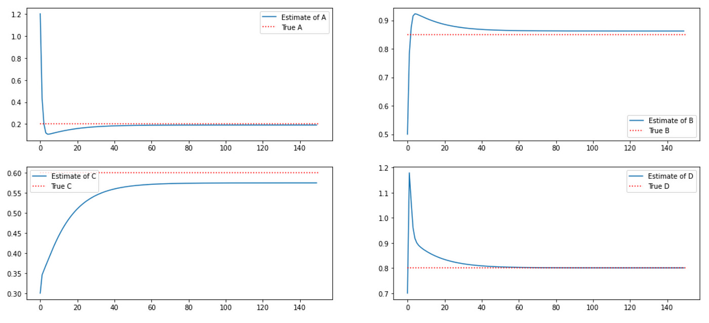
So it seems that we were able to successfully implement EM algorithm for estimating model parameters. Now let’s see if it can be used for trading.
The paper doesn’t say anything about selecting pairs for trading. It just says that if coefficient B is between 0 and 1, then it is consistent with mean reverting model. Another condition is mentioned in section 2.2. It says that parameter C must be less than parameter D. I’m going to use these two conditions as well.
Another question is the size of sliding window on which we should estimate model parameters. No suggestions are made in the paper, so I’m going to make a guess and use a window of 30 trading days, which is approximately 1.5 months.
After spread model parameters are estimated we need to determine which trading strategy to use. Two trading strategies are proposed in the paper.
First one suggests to compare observed spread price with the price predicted by Kalman filter. It seems easy at first glance, but details are confusing to me. First of all, which variables should we compare? If I correctly understand notation in the paper, they suggest to compare the prediction of the spread price from the previous time step with the observed spread price from the current time step. I don’t understand why we should do that. Why use estimate from the previous time step if we already have estimate at the current time step and moreover we can use our model to make a prediction of the price in the next time step. Another thing that I don’t understand is why it is suggested to enter a long position when the observed price is too high (higher than the estimate) and enter a short position if the observed price is too low (lower than the estimate). It seems logical to me that we should do exactly the opposite: short the spread if it is too high and long if it is too low. I’d think that this is just a typo, but another paper (based on the results of the one I’m trying to implement) suggests the same (see section 4.5). It is highly unlikely that two papers would have the same mistake, but I don’t understand what is wrong with my reasoning.
The second proposed strategy suggests the following thresholds for entering positions:
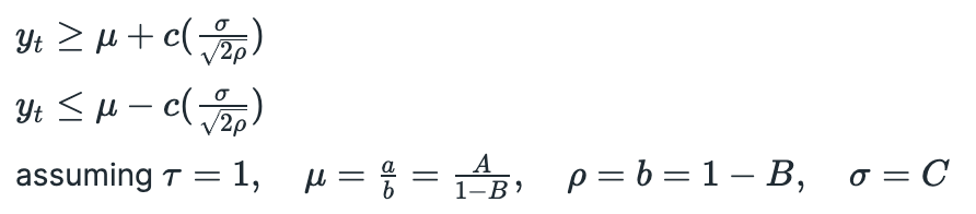
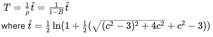
The value of parameter c is not specified and nothing is said about which condition we should use for long and which for short positions. Positions are closed at time T — First Passage Time of Ornstein-Uhlenbeck process, which is calculated as follows:
Now we are ready to backtest both strategies.
I will use daily prices of some biotech stocks and ETFs (I used the same dataset in some of my previous posts). First I will perform parameter estimation and selecting mean reverting pairs. I will use 30 days sliding window and on each trading day do the following:
estimate parameters A,B,C,D of all possible pairs of assets
choose pairs that satisfy the conditions 0<B<1 and 0<C<D
save selected pairs and their parameters
Below you can see the code I used to perform the described procedures.
| good_pairs_all = {} | |
| window = 30 | |
| for i in range(window,len(cumret_norm.index)): | |
| print(f'Processing day {i-window}') | |
| cumret_tmp_prev = cumret_norm.iloc[i-window:i,] # data for parameter estimation | |
| # estimate parameters | |
| ip = {'A':2, 'B':2, 'C':2, 'D':2} # initial parameters | |
| tested_pairs = [] | |
| good_pairs = {} | |
| for s1 in cumret_tmp_prev.columns: | |
| for s2 in cumret_tmp_prev.columns: | |
| if s1!=s2 and (f'{s1}-{s2}' not in tested_pairs) and (f'{s2}-{s1}' not in tested_pairs): | |
| tested_pairs.append(f'{s1}-{s2}') | |
| spread = cumret_tmp_prev[s1] - cumret_tmp_prev[s2] | |
| params = ss_smoother(spread, ip, num_iter=150, x_0=spread.iloc[0], R_0=ip['D']) | |
| params = {k:v[-1] for k,v in params.items()} | |
| if params['B']>0 and params['B']<1: | |
| if params['C'] < params['D']: | |
| good_pairs[f'{s1}-{s2}'] = params # save pair and parameters | |
| # save pairs and parameters | |
| pairs_df = pd.DataFrame.from_dict(good_pairs, orient='index') | |
| date = cumret_tmp_prev.index[-1] | |
| good_pairs_all[date] = pairs_df |
This procedure takes quite some time to complete, so I saved the resulting dictionary as a Python pickle. You can download it here.
Now we are ready to test the strategies. I will test modifications of the proposed strategies, which are a little bit easier to implement and which should give us a basic idea wether we should spend time trying to optimize them.
For the first trading strategy the algorithm will be as follows:
Using estimated parameters of the spread run Kalman filter on last N datapoints (N=30 in my case)
Long pairs for which observed spread price is bigger than the Kalman filter estimate
Short pairs for which observed spread price is lower than the Kalman filter estimate
Close and recalculate positions each trading day
In practice we would need to use some thresholds for opening and closing positions, but the version described above is easier to implement and it can give us a general idea about the performance of the strategy.
We should make one more decision. Which estimate should we compare to the observed price? First I’ll use the one suggested in the paper — predicted price from the previous time step. Then I’ll try another approach, which seems more reasonable to me — predicted price for the next time step using current estimate.
Approach #1
I will follow the rules described in the paper: go long when the observed price is smaller than the predicted price from the previous time step, and go short when the observed price is lower than the predicted price from the previous time step. The code I used and cumulative return plot are provided below.
| with open('spread_params.pkl', 'rb') as f: | |
| good_pairs_all = pickle.load(f) | |
| selected_pairs_long = [] | |
| selected_pairs_short = [] | |
| algo_ret = [] | |
| num_days = len(cumret_norm.index) | |
| for i in range(30,num_days): | |
| cumret_tmp = cumret_norm.iloc[i-30:i] | |
| ret_tmp = returns.iloc[i-1] | |
| # calculate returns | |
| daily_returns_long = [] | |
| daily_returns_short = [] | |
| if len(selected_pairs_long)>0: | |
| for pair in selected_pairs_long: | |
| s1,s2 = parse_pair(pair) | |
| daily_returns_long.append(ret_tmp[s1] - ret_tmp[s2]) | |
| selected_pairs_long = [] | |
| if len(selected_pairs_short)>0: | |
| for pair in selected_pairs_short: | |
| s1,s2 = parse_pair(pair) | |
| daily_returns_short.append(-ret_tmp[s1] + ret_tmp[s2]) | |
| selected_pairs_short = [] | |
| # equal capital allocations to longs\shorts | |
| daily_return_total = np.mean(daily_returns_long) + np.mean(daily_returns_short) | |
| algo_ret.append(daily_return_total) | |
| date = returns.index[i-1] | |
| if len(good_pairs_all[date].index)>0: | |
| # calculate spreads | |
| pairs_df = good_pairs_all[date] | |
| for pair in pairs_df.index: | |
| s1,s2 = parse_pair(pair) | |
| params = pairs_df.loc[pair] | |
| observed_spread = (cumret_tmp[s1] - cumret_tmp[s2]).values | |
| yesterday_pred, today_est = kalman_filter(observed_spread, params) | |
| pairs_df.loc[pair, ['spread_pred']] = yesterday_pred # x_{k|k-1} | |
| pairs_df.loc[pair, ['y']] = observed_spread[-1] # y_k | |
| pairs_df['current-predicted'] = pairs_df['y'] - pairs_df['spread_pred'] | |
| selected_pairs_long = pairs_df[pairs_df['current-predicted']>0].index | |
| selected_pairs_short = pairs_df[pairs_df['current-predicted']<0].index |
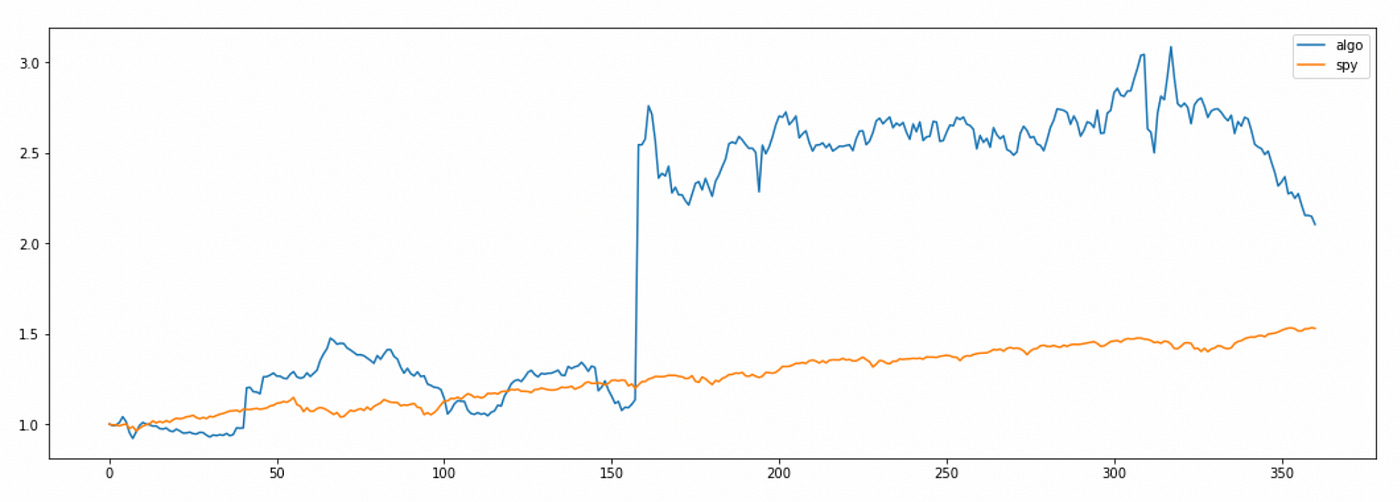
The total return of the algorithm looks quite good, but we can see that most of the profit is made on one ‘lucky’ day in the middle of the tested time period. Also note that algorithm returns are very volatile.
Approach #2
Now I will try to use predicted price for the next period as an estimate. Source code and cumulative returns plot are provided below.
| with open('spread_params.pkl', 'rb') as f: | |
| good_pairs_all = pickle.load(f) | |
| selected_pairs_long = [] | |
| selected_pairs_short = [] | |
| algo_ret = [] | |
| num_days = len(cumret_norm.index) | |
| for i in range(30,num_days): | |
| cumret_tmp = cumret_norm.iloc[i-30:i] | |
| ret_tmp = returns.iloc[i-1] | |
| # calculate returns | |
| daily_returns_long = [] | |
| daily_returns_short = [] | |
| if len(selected_pairs_long)>0: | |
| for pair in selected_pairs_long: | |
| s1,s2 = parse_pair(pair) | |
| daily_returns_long.append(ret_tmp[s1] - ret_tmp[s2]) | |
| selected_pairs_long = [] | |
| if len(selected_pairs_short)>0: | |
| for pair in selected_pairs_short: | |
| s1,s2 = parse_pair(pair) | |
| daily_returns_short.append(-ret_tmp[s1] + ret_tmp[s2]) | |
| selected_pairs_short = [] | |
| # equal capital allocations to longs\shorts | |
| daily_return_total = np.mean(daily_returns_long) + np.mean(daily_returns_short) | |
| algo_ret.append(daily_return_total) | |
| date = returns.index[i-1] | |
| if len(good_pairs_all[date].index)>0: | |
| # calculate spreads | |
| pairs_df = good_pairs_all[date] | |
| for pair in pairs_df.index: | |
| s1,s2 = parse_pair(pair) | |
| params = pairs_df.loc[pair] | |
| observed_spread = (cumret_tmp[s1] - cumret_tmp[s2]).values | |
| yesterday_pred, today_est = kalman_filter(observed_spread, params) | |
| pairs_df.loc[pair, ['spread_est']] = today_est # x_{k|k} | |
| pairs_df.loc[pair, ['y']] = observed_spread[-1] # y_k | |
| pairs_df['spread_pred_tom'] = pairs_df['A'] + pairs_df['B'] * pairs_df['spread_est'] | |
| pairs_df['current-predicted_tom'] = pairs_df['y'] - pairs_df['spread_pred_tom'] | |
| selected_pairs_long = pairs_df[pairs_df['current-predicted_tom']>0].index | |
| selected_pairs_short = pairs_df[pairs_df['current-predicted_tom']<0].index |
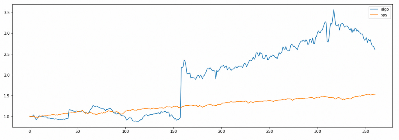
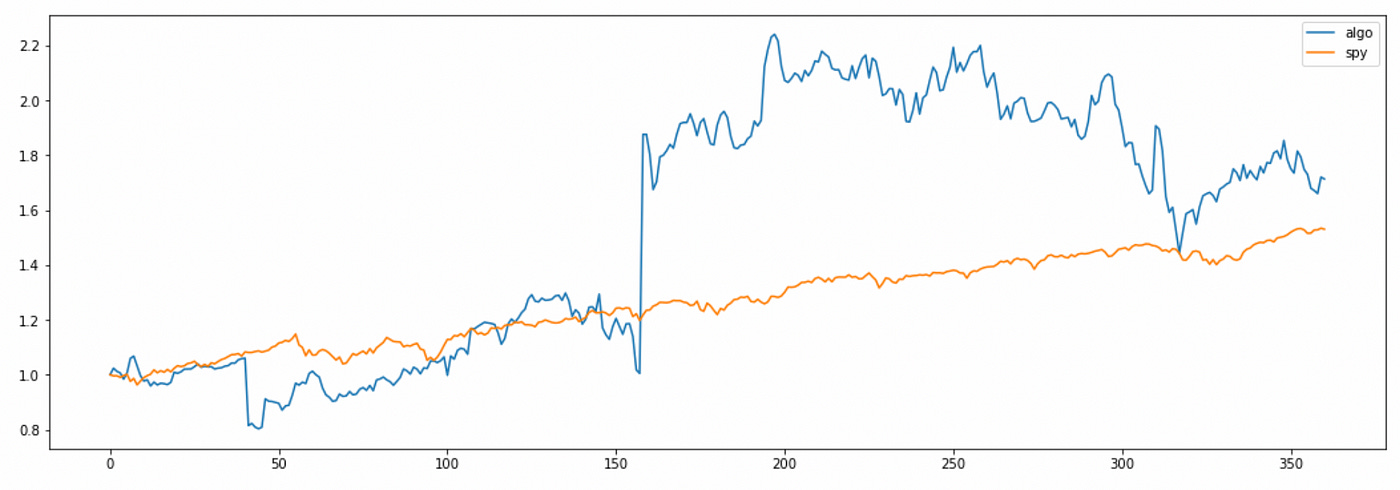
Here again algorithm returns are very volatile, but total return is even better than before.
I want to emphasize again that the rules for entering long\short positions I used here are the ones that are described in the paper. They make no sense to me. I don’t understand why we go long on the spread which is too expensive and go short on the spread that is too cheap. But these rules seem to work (although it might be just a fluke).
Now let’s try backtesting another strategy. To simplify it I assume that c=0 and open a long positions when observed price is less than the mean and go short when observed price is greater than the mean. The first passage time won’t be important here because the parameters are recalculated each day and we know which pairs are mispriced given the current information. So it is just a small modification of the first strategy.
| with open('spread_params.pkl', 'rb') as f: | |
| good_pairs_all = pickle.load(f) | |
| selected_pairs_long = [] | |
| selected_pairs_short = [] | |
| algo_ret = [] | |
| num_days = len(cumret_norm.index) | |
| c = 0 | |
| for i in range(30,num_days): | |
| cumret_tmp = cumret_norm.iloc[i-30:i] | |
| ret_tmp = returns.iloc[i-1] | |
| # calculate returns | |
| daily_returns_long = [] | |
| daily_returns_short = [] | |
| if len(selected_pairs_long)>0: | |
| for pair in selected_pairs_long: | |
| s1,s2 = parse_pair(pair) | |
| daily_returns_long.append(ret_tmp[s1] - ret_tmp[s2]) | |
| selected_pairs_long = [] | |
| if len(selected_pairs_short)>0: | |
| for pair in selected_pairs_short: | |
| s1,s2 = parse_pair(pair) | |
| daily_returns_short.append(-ret_tmp[s1] + ret_tmp[s2]) | |
| selected_pairs_short = [] | |
| # equal capital allocations to longs\shorts | |
| daily_return_total = np.mean(daily_returns_long) + np.mean(daily_returns_short) | |
| algo_ret.append(daily_return_total) | |
| date = returns.index[i-1] | |
| if len(good_pairs_all[date].index)>0: | |
| # calculate spreads | |
| pairs_df = good_pairs_all[date] | |
| for pair in pairs_df.index: | |
| s1,s2 = parse_pair(pair) | |
| params = pairs_df.loc[pair] | |
| observed_spread = (cumret_tmp[s1] - cumret_tmp[s2]).values | |
| pairs_df.loc[pair, ['y']] = observed_spread[-1] # y_k | |
| # calculate mu, rho, and sigma | |
| pairs_df['mu'] = pairs_df['A'] / (1 - pairs_df['B']) | |
| pairs_df['rho'] = 1 - pairs_df['B'] | |
| pairs_df['sigma'] = pairs_df['C'] | |
| # calculate upper\lower thresholds | |
| pairs_df['upper'] = pairs_df['mu'] + c * pairs_df['sigma'] / np.sqrt(2 * pairs_df['rho']) | |
| pairs_df['lower'] = pairs_df['mu'] - c * pairs_df['sigma'] / np.sqrt(2 * pairs_df['rho']) | |
| selected_pairs_long = pairs_df[pairs_df['y'] < pairs_df['lower']].index | |
| selected_pairs_short = pairs_df[pairs_df['y'] > pairs_df['upper']].index |
As you can see above, the total return of the strategy is a little higher than the return of the market, but a lot more volatile. Also note that the rules for entering long\short positions make more sense here: I buy the spread if its price is too low and I sell the spread if its price is too high.
First two strategies give us good total return, but we need to take into account the fact that most of the profit is made on one day and that I didn’t any include transaction costs. Additionally, there might be some ways to improve the performance even more:
Allow non-equal capital allocation to assets in a pair when forming the spread (use simple linear regression to calculate hedge ratio)
Select only pairs which are expected to converge soon enough (set some threshold for the First Passage Time of OU-process)
Use higher frequency data
Use different sliding window size
Use larger selection of stocks (or try using stocks from more stable industries than biotechnology)
Select optimal thresholds for entering and exiting positions
Jupyter notebook with source code is available here.
If you have any questions, suggestions or corrections please post them in the comments. Thanks for reading.
Hi, why didn't you model the spread with a cointegration coefficient? Wouldn't this be more theoretically aligned? And how important is the parameter constraint of C < D when dealing with daily price data really? I noticed that when I relax this constraint, many more pairs pass the constraints (0 < B < 1, C >= 0 and D > 0).