Pairs trading with copulas
Trying to capture complex dependencies in financial markets.

Two previous articles were dedicated to describing the general idea behind copula and different copula families. Now we can apply these ideas to implementing a pairs trading strategy. In this article I am going to implement and backtest a strategy based on paper ‘Trading strategies with copulas’ by Stander at al. (2013).
The general algorithm is this:
Select pairs for trading
Fit marginal distribution for returns of each stock in the pair (either parametric of empirical)
Use probability integral transform to make marginal returns uniformly distributed
Fit copula to transformed returns
Use fitted copula to calculate conditional probabilities
Enter long\short positions when conditional probabilities fall outside predefined confidence bands (I will describe trading rules in more detail later)
We start with selecting stocks and pairs for trading. I will use constituents of Vanguard Small-Cap Value ETF (ticker: VBR) as my universe of stocks. The time period will be from 2018–11–20 to 2021–11–19. I am going to use first 30 months as formation period and last 6 months as trading period.
First step is identifying potential pairs for trading. I will select pairs with the highest Kendall’s rank correlation coefficient (Kendall’s tau) between log-returns. There are 256686 possible pairs and computing correlation for each pair takes some time. I provide the results of this computation in a csv file here, so that you don’t have to do it.
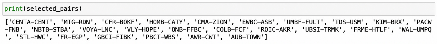
I am going to select 25 pairs with the highest Kendall’s tau (and consisting of different stocks). So if potential pair contains a stock that is already selected as a part of another pair, I’ll drop such pair and proceed to the next. Code for pair selection is shown below.
| # load data | |
| prices = pd.read_csv('vbr18_21.csv', index_col=0) | |
| prices = prices.dropna(axis=1) | |
| returns = np.log(prices).diff().dropna() | |
| form_start = '2018-11-20' | |
| form_end = '2020-05-19' | |
| trade_start = '2021-05-20' | |
| trade_end = '2021-11-19' | |
| prices_form = prices[form_start:form_end] | |
| prices_trade = prices[trade_start:trade_end] | |
| returns_form = returns.loc[form_start:form_end] | |
| returns_trade = returns.loc[trade_start:trade_end] | |
| # Calculate Kendall's tau for each pair of stocks | |
| results = pd.DataFrame(columns=['tau']) | |
| for s1 in returns_form.columns: | |
| for s2 in returns_form.columns: | |
| if (s1!=s2) and (f'{s2}-{s1}' not in results.index): | |
| results.loc[f'{s1}-{s2}'] = stats.kendalltau(returns_form[s1], returns_form[s2])[0] | |
| def parse_pair(pair): | |
| s1 = pair[:pair.find('-')] | |
| s2 = pair[pair.find('-')+1:] | |
| return s1,s2 | |
| # select pairs | |
| selected_stocks = [] | |
| selected_pairs = [] | |
| for pair in results.sort_values(by='tau', ascending=False).index: | |
| s1,s2 = parse_pair(pair) | |
| if (s1 not in selected_stocks) and (s2 not in selected_stocks): | |
| selected_stocks.append(s1) | |
| selected_stocks.append(s2) | |
| selected_pairs.append(pair) | |
| if len(selected_pairs) == 25: | |
| break |
Let’s have a look at the selected pairs:
Now we can try and fit marginal distributions to log-returns data. I will try fitting four parametric distributions: normal, Student’s t, logistic and extreme. The selection will be made based on Akaike Information Criterion(AIC). For selected distribution I will also compute Bayesian Information Criterion (BIC) and p-value of Kolmogorov-Smirnov goodness-of-fit test.
| marginals_df = pd.DataFrame(index=selected_stocks, columns=['Distribution', 'AIC', 'BIC', 'KS_pvalue']) | |
| for stock in selected_stocks: | |
| data = returns_form[stock] | |
| dists = ['Normal', "Student's t", 'Logistic', 'Extreme'] | |
| best_aic = np.inf | |
| for dist,name in zip([stats.norm, stats.t, stats.genlogistic, stats.genextreme], dists): | |
| params = dist.fit(data) | |
| dist_fit = dist(*params) | |
| log_like = np.log(dist_fit.pdf(data)).sum() | |
| aic = 2*len(params) - 2 * log_like | |
| if aic<best_aic: | |
| best_dist = name | |
| best_aic = aic | |
| best_bic = len(params) * np.log(len(data)) - 2 * log_like | |
| ks_pval = stats.kstest(data, dist_fit.cdf, N=100)[1] | |
| marginals_df.loc[stock] = [best_dist, best_aic, best_bic, ks_pval] |
Let’s look at the first few rows of resulting dataframe.
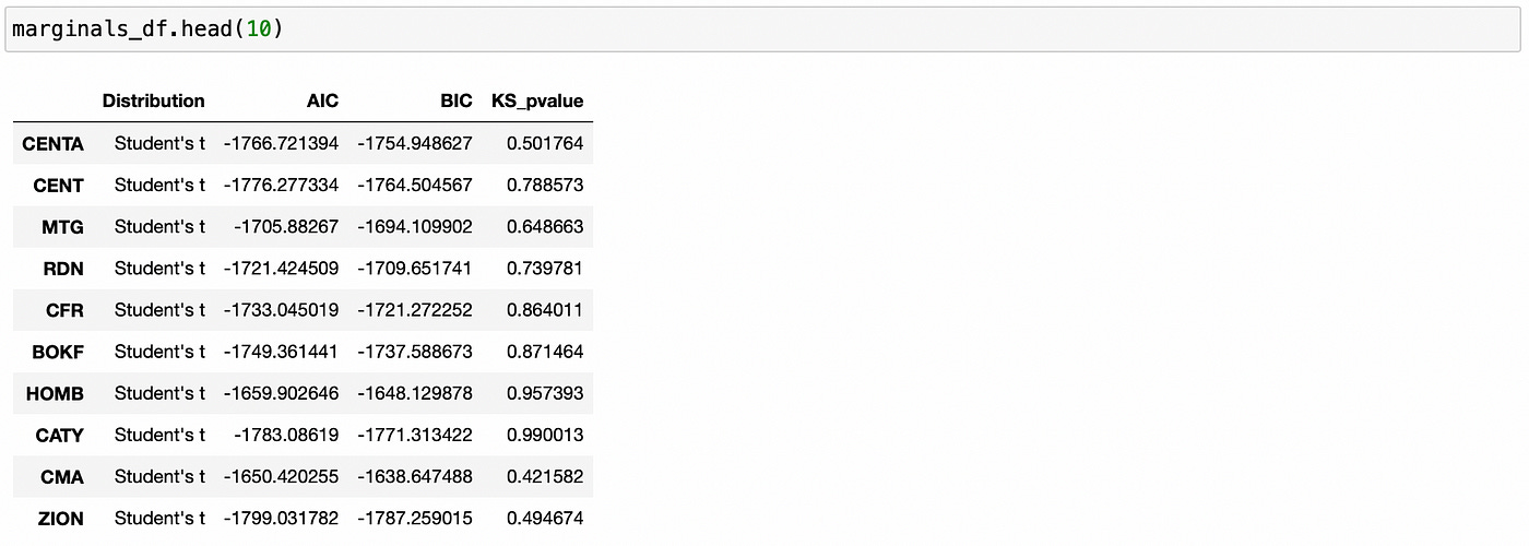
For all the stocks above Student’s t distribution was selected. P-values of Kolmogorov-Smirnov test are quite large, meaning that we can’t reject the null hypothesis that tested distributions are the same. That allows us to conclude that selected parametric distributions model empirical data sufficiently well.
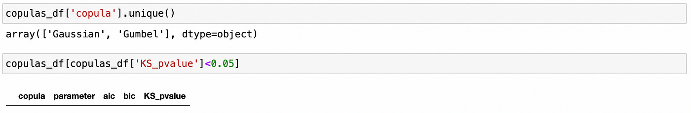
Let’s see if any other distribution families were selected for other stocks.

No, Student’s t family is the best fit for all of the stocks.
Now let’s see if there are any stocks with low KS-test p-values (meaning that the selected parametric distribution is not a good fit).

No, seems that we are able to model all returns quite well. Now we can proceed to fitting copulas.
I am going to reuse the code I wrote for previous two articles on copulas. I made some changes and created classes for all copula families, but basically it’s the same code in a different wrap. Everything is saved in separate file (copulas.py), which I import in line 1. Another thing I need is two-dimensional Kolmogorov-Smirnov test, which is not implemented in scipy. I am using an implementation found here. It is imported in line 2. Everything else should be clear from the code:
Fit marginal distributions (using only Student’s t distribution family)
Apply probability integral transform to marginal returns (by plugging returns into selected distribution’s cdf)
Fit each copula family (Gaussian, Clayton, Gumbel, Frank, Joe) and compute AIC
Select copula with the smallest AIC and calculate its BIC and KS-test p-value
| from copulas import * | |
| import ndtest # bivariate Kolmogorov-Smirnov | |
| copulas_df = pd.DataFrame(index=selected_pairs, columns=['copula', 'parameter', 'aic', 'bic', 'KS_pvalue']) | |
| for pair in selected_pairs: | |
| s1,s2 = parse_pair(pair) | |
| # fit marginals | |
| params_s1 = stats.t.fit(returns_form[s1]) | |
| dist_s1 = stats.t(*params_s1) | |
| params_s2 = stats.t.fit(returns_form[s2]) | |
| dist_s2 = stats.t(*params_s2) | |
| # apply probability integral transform | |
| u = dist_s1.cdf(returns_form[s1]) | |
| v = dist_s2.cdf(returns_form[s2]) | |
| best_aic = np.inf | |
| for copula in [GaussianCopula(), ClaytonCopula(), GumbelCopula(), FrankCopula(), JoeCopula()]: | |
| copula.fit(u,v) | |
| L = copula.log_likelihood(u,v) | |
| aic = 2 * copula.num_params - 2 * L | |
| if aic < best_aic: | |
| best_aic = aic | |
| best_bic = copula.num_params * np.log(len(u)) - 2 * L | |
| best_copula = copula.name | |
| # calculate KS-pvalue | |
| smp = copula.sample(size=len(u)) # generate sample from fit copula | |
| s_u = smp[:,0] | |
| s_v = smp[:,1] | |
| ks_pval = ndtest.ks2d2s(u,v,s_u,s_v) | |
| if isinstance(copula, ArchimedeanCopula): | |
| best_param = copula.alpha | |
| else: | |
| best_param = copula.rho | |
| copulas_df.loc[pair] = [best_copula, best_param, best_aic, best_bic, ks_pval] |
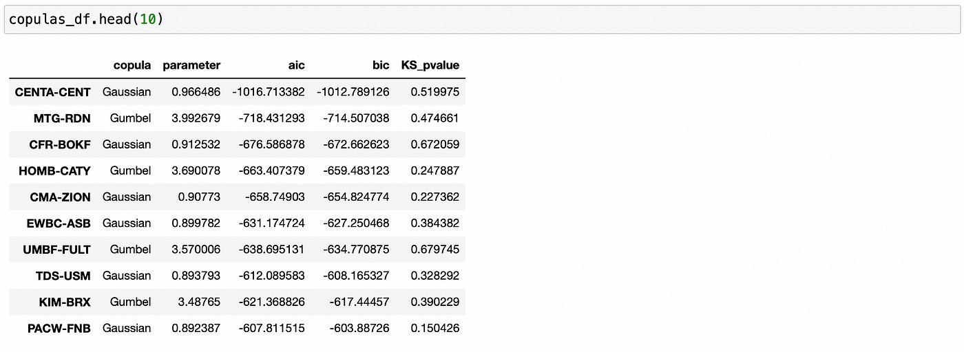
We can see above (from KS-test p-values) that selected copulas provide a good fit for the empirical data. We can also check if any other copula families were selected for other pairs and if any pairs have low p-values of KS-test.
In the paper authors try to fit all 22 different families of Archimedean copulas listed and Roger B. Nelsen’s book ‘An introduction to copulas’. I wasn’t able to find a library for Python with all Archimedean copulas implemented, so I decided to only use a limited number of copulas I implemented myself.
Now we need to define trading rules. Remember that we are trading in a spread — buying one stock and simultaneously selling another. So we need to know when one stock is underpriced and another stock is overpriced. That’s where copula can help.
First we need to calculate conditional probabilities:
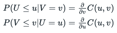
It is not necessary to solve these equations analytically. I have implemented class methods to compute conditional probabilities numerically from a random sample. Now we just need to plug returns into respective marginal CDF (apply probability integral transform to transform returns to standard uniform distribution) and we are ready to calculate conditional probabilities. If calculated probability is too low, then the stock is underpriced, it calculated probability is too high, then the stock is overpriced. Conditions for opening long\short positions are presented below. Random variables Uand V represent transformed returns of each stock in the pair and c is called a confidence level.
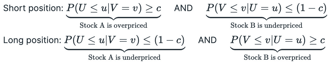
In many other pairs trading strategies decisions are made based on the price (or return) of the spread. If the spread was mispriced we automatically assumed that one stock must be too high and another is too low (or vice versa). Here we explicitly check both conditions: that one stock is overpriced and another is underpriced. Both conditions must be true for us to open a position.
According to the paper, we should ‘exit the trade when the two stocks revert to their historical relationship’, but no specific rules are provided. In another paper (Liew and Wu, 2013) positions are closed when the conditional probabilities cross the boundary of 0.5. I’m going to use that rule in my backtest.
Probably these rules not seem very clear now, but it’ll be easier to understand from the code below.
| algo_returns = {} | |
| cl = 0.99 # confidence level | |
| for pair in selected_pairs: | |
| s1,s2 = parse_pair(pair) | |
| # fit marginals | |
| params_s1 = stats.t.fit(returns_form[s1]) | |
| dist_s1 = stats.t(*params_s1) | |
| params_s2 = stats.t.fit(returns_form[s2]) | |
| dist_s2 = stats.t(*params_s2) | |
| # transform marginals | |
| u = dist_s1.cdf(returns_form[s1]) | |
| v = dist_s2.cdf(returns_form[s2]) | |
| # fit copula | |
| best_aic = np.inf | |
| best_copula = None | |
| copulas = [GaussianCopula(), ClaytonCopula(), GumbelCopula(), FrankCopula(), JoeCopula()] | |
| for copula in copulas: | |
| copula.fit(u,v) | |
| L = copula.log_likelihood(u,v) | |
| aic = 2 * copula.num_params - 2 * L | |
| if aic < best_aic: | |
| best_aic = aic | |
| best_copula = copula | |
| # calculate conditional probabilities | |
| prob_s1 = [] | |
| prob_s2 = [] | |
| for u,v in zip(dist_s1.cdf(returns_trade[s1]), dist_s2.cdf(returns_trade[s2])): | |
| prob_s1.append(best_copula.cdf_u_given_v(u,v)) | |
| prob_s2.append(best_copula.cdf_v_given_u(u,v)) | |
| probs_trade = pd.DataFrame(np.vstack([prob_s1, prob_s2]).T, index=returns_trade.index, columns=[s1, s2]) | |
| # calculate positions | |
| positions = pd.DataFrame(index=probs_trade.index, columns=probs_trade.columns) | |
| long = False | |
| short = False | |
| for t in positions.index: | |
| # if long position is open | |
| if long: | |
| if (probs_trade.loc[t][s1] > 0.5) or (probs_trade.loc[t][s2] < 0.5): | |
| positions.loc[t] = [0,0] | |
| long = False | |
| else: | |
| positions.loc[t] = [1,-1] | |
| # if short position is open | |
| elif short: | |
| if (probs_trade.loc[t][s1] < 0.5) or (probs_trade.loc[t][s2] > 0.5): | |
| positions.loc[t] = [0,0] | |
| short = False | |
| else: | |
| positions.loc[t] = [-1,1] | |
| # if no positions are open | |
| else: | |
| if (probs_trade.loc[t][s1] < (1-cl)) and (probs_trade.loc[t][s2] > cl): | |
| # open long position | |
| positions.loc[t] = [1,-1] | |
| long = True | |
| elif (probs_trade.loc[t][s1] > cl) and (probs_trade.loc[t][s2] < (1-cl)): | |
| # open short positions | |
| positions.loc[t] = [-1,1] | |
| short = True | |
| else: | |
| positions.loc[t] = [0,0] | |
| # calculate returns | |
| algo_ret = (returns_trade * positions.shift()).sum(axis=1) | |
| algo_returns[pair] = algo_ret |
I process each pair separately and do the following:
Fit marginal distribution for each stock in the pair
Transform marginal returns into standard uniform distribution using probability integral tranfsorm
Fit copula on transformed returns (all steps up to this are performed on formation period data)
Calculate conditional probabilities for each day in trading period (using marginals and copula from the previous steps)
Create positions dataframe according to the rules described above
Calculate algorithm returns
After running that code, we have a dictionary with returns for each individual pair. Recall that we were using log-returns and they need to be transformed back to simple returns.
To calculate total returns we sum daily returns of each pair and divide it by total number of traded pairs (assuming equal capital allocation to each pair). We also multiply total return by 2 since we can use cash from short positions to open long positions. Below you can see the code for calculating and plotting returns. I also plot returns of VBR ETF for comparison.
| returns = pd.DataFrame.from_dict(algo_returns) | |
| returns = np.exp(returns) - 1 # convert log-returns to simple returns | |
| total_ret = returns.sum(axis=1) / len(returns.columns) * 2 # double capital (from short positions) | |
| import yfinance as yf | |
| vbr_price = yf.download('VBR', start=trade_start, end=trade_end) | |
| vbr_price = vbr_price['Adj Close'] | |
| vbr_ret = vbr_price.pct_change().dropna() | |
| plt.figure(figsize=(18,6)) | |
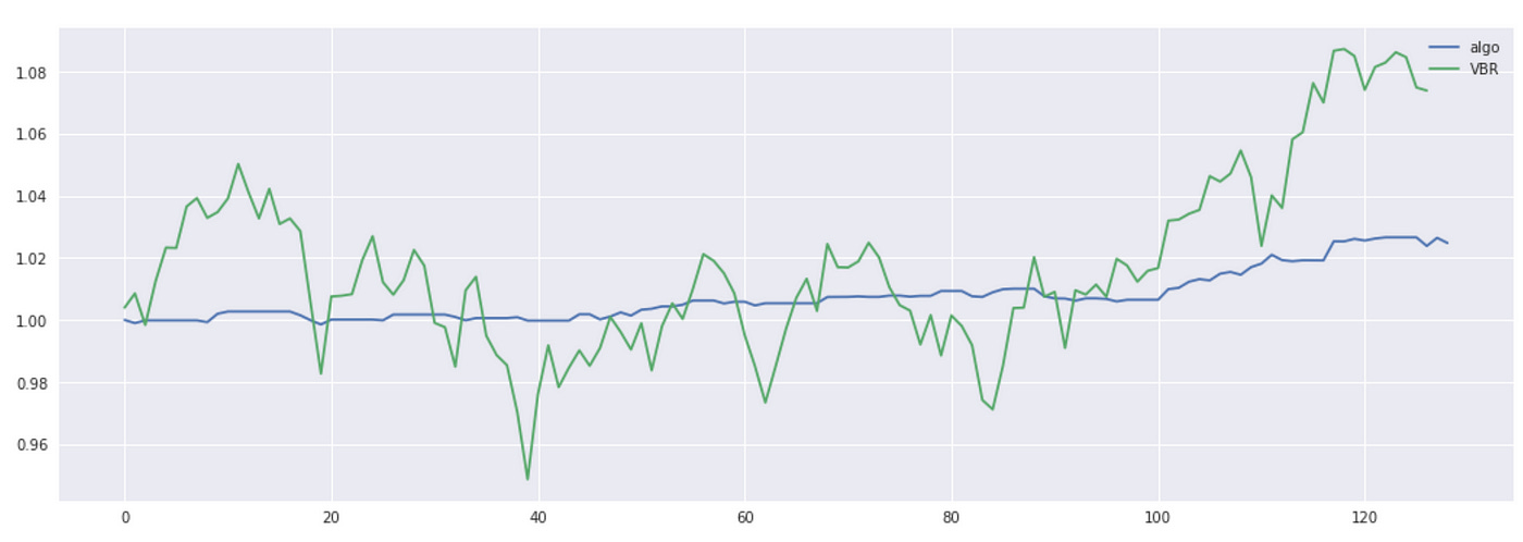
| plt.plot(np.nancumprod(total_ret + 1), label='algo') | |
| plt.plot(np.nancumprod(vbr_ret + 1), label='VBR') | |
| plt.legend() |
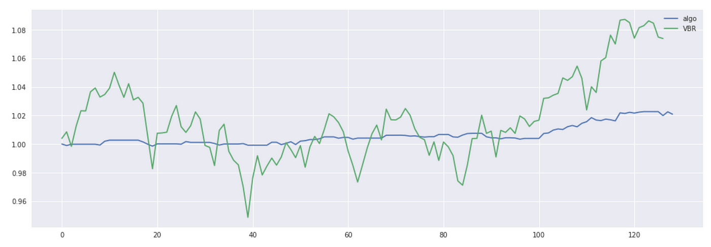
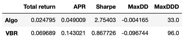
The total return is quite small, but we can see that algorithm returns are a lot less volatile. Let’s look at some metrics.
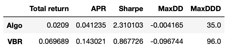
Even though the total return is not high, the Sharpe ratio of out algorithm is very good and its maximum drawdown is only 0.4% compared to 9.6% drawdown of VBR. Please note that here I didn’t account for any transaction costs.
Let’s try a little modification of this strategy and see what happens when we exit positions earlier. Instead of using conditional probability boundary of 0.5, I will use a boundary of 0.3 for long positions and 0.7 for short positions. We only need to modify one part of the code (where we define rules for exiting positions):
| for t in positions.index: | |
| # if long position is open | |
| if long: | |
| if (probs_trade.loc[t][s1] > 0.3) or (probs_trade.loc[t][s2] < 0.7): | |
| positions.loc[t] = [0,0] | |
| long = False | |
| else: | |
| positions.loc[t] = [1,-1] | |
| # if short position is open | |
| elif short: | |
| if (probs_trade.loc[t][s1] < 0.7) or (probs_trade.loc[t][s2] > 0.3): | |
| positions.loc[t] = [0,0] | |
| short = False | |
| else: | |
| positions.loc[t] = [-1,1] |
Plot of the cumulative returns and performance metrics are shown below.
We get a slight increase in APR and Sharpe ratio, but I can’t say that we got any significant improvement.
Overall I think that the results we got are not that bad. It might be possible to improve the performance of the strategy by making some modifications. Some ideas to test:
Use better methods of pair selection.
Implement and try to fit more different copulas.
Update pairs (or at least refit marginal distributions and copulas) more often.
Derive better rules for closing positions.
Use higher frequency data.
Jupyter notebook with source code is available here.
If you have any questions, suggestions or corrections please post them in the comments. Thanks for reading.