

Portfolio optimization with factor models
Using factor models for improving covariance matrix estimation.

Recall from my previous articles on portfolio optimization that the sample covariance matrix is very noisy and the more assets there are in our trading universe, the more noise we have in our sample covariance matrix. If we have a dataset with daily returns of 500 stocks spanning one year, it contains approximately 250*500=125000 datapoints. To estimate covariance matrix we need to calculate covariance for 500*499/2=124750 pairs of stocks. With roughly one data point per parameter, it's not surprising that the sample covariance matrix is noisy.
In this article, I aim to improve covariance matrix estimates with factor models. Factor models allow us to represent asset returns as a function of a few common variables (factors), reducing the complexity of covariance estimation. This can lead to more stable covariance estimates, ultimately improving the performance of portfolio optimization strategies.
First, let’s backtest a couple of baseline strategies, which we will use later for comparison. For this purpose, I’m going to use market-weighted portfolio (represented by SPY) and equally weighted portfolio. Code for loading data and backtesting these strategies is provided below.
| prices = pd.read_csv('sp500.csv', index_col=0) | |
| returns = prices.pct_change().dropna() | |
| spy = yf.download('SPY', start='2018-01-01', end='2023-01-01') | |
| spy_price = spy['Adj Close'] | |
| spy_ret = spy['Adj Close'].pct_change().dropna() | |
| returns.index = spy_ret.index | |
| # prepare weekly data | |
| prices.index = pd.to_datetime(prices.index) | |
| prices_w = prices.resample('1W').last() | |
| returns_w = prices_w.pct_change().dropna() | |
| spy_price_w = spy_price.resample('1W').last() | |
| spy_ret_w = spy_price_w.pct_change().dropna() | |
| # calculate cumulative returns | |
| cumret_eqw = (1 + returns_w.loc['2019-01-01':].sum(axis=1)/returns.shape[1]).cumprod() | |
| cumret_spy = (1 + spy_ret_w.loc['2019-01-01':]).cumprod() | |
| # calculate performance metrics | |
| results_df = pd.DataFrame(columns = ['Total return', 'APR', 'Sharpe', 'MaxDD', 'MaxDDD']) | |
| results_df.loc['SPY'] = calculate_metrics(cumret_spy) | |
| results_df.loc['Equally Weighted'] = calculate_metrics(cumret_eqw) |
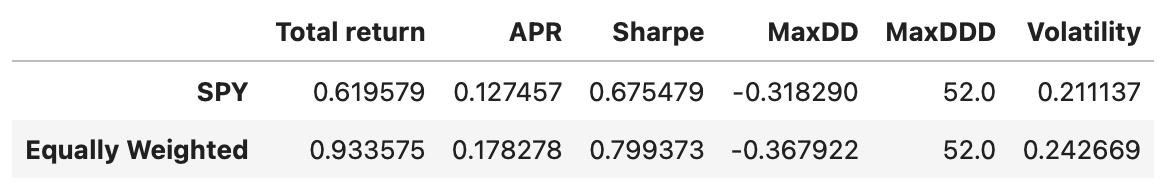
Last column of the table above shows annualized volatility of strategy returns. Volatility of the equally weighted portfolio will be used as a target volatility in portfolio optimization.
Now we are ready to test strategies based on portfolio optimization techniques. Here’s a summary of the trading strategy I’m going to use.
Trading universe: SP500 constituents.
Time period: from 2019-01-01 to 2022-12-31.
Rebalancing: weekly.
Trading rules:
Each week, a new target portfolio is calculated by solving a portfolio optimization problem.
The optimization goal is to maximize expected returns for a given level of volatility.
The target volatility is set to match the volatility of an equally weighted portfolio.
Expected returns and covariance matrix are estimated using daily returns data over a one-year trailing window (252 trading days).
I’ve used a similar strategy in my previous articles on portfolio optimization. The only things that change are the trading universe and the techniques for estimating covariance matrix.
Let’s begin by backtesting a strategy that uses sample covariance matrix. First, we need to define a few functions and variables (described in more detail in my previous articles on portfolio optimization).
| # find minimum variance portfolio | |
| from scipy.optimize import minimize | |
| # function to minimize | |
| def volatility(weights, returns_covariance): | |
| return np.sqrt(weights.T @ returns_covariance @ weights * 252) | |
| def negative_annual_return(weights, returns_mean): | |
| ret = weights.T @ returns_mean * 252 | |
| return -ret | |
| stocks = returns.columns | |
| # initial guess | |
| x0 = np.ones(len(stocks)) / len(stocks) | |
| # bounds | |
| bounds=[[0,1]]*len(stocks) |
The code for backtesting is also similar to the previous articles.
| positions = pd.DataFrame(index=returns_w.loc['2019-01-01':].index, columns=returns_w.columns) | |
| target_vol = volatility_eqw | |
| bounds=[[0,1]]*len(stocks) | |
| x0 = np.ones(len(stocks)) / len(stocks) | |
| for t in tqdm(returns_w.loc['2019-01-01':].index): | |
| # prepare data | |
| prices_tmp = prices.loc[:t].iloc[-252:] | |
| returns_tmp = prices_tmp.pct_change().dropna() | |
| # perform optimization | |
| constraints = ({'type':'eq', 'fun': lambda x: volatility(x,returns_tmp.cov())-target_vol}, | |
| {'type':'eq', 'fun': lambda x: np.sum(x)-1}) | |
| res = minimize(negative_annual_return, x0, args=(returns_tmp.mean()), | |
| bounds=bounds, constraints=constraints) | |
| if res.status!=0: | |
| print('Optimization failed') | |
| positions.loc[t] = positions.loc[:t].iloc[-2] # keep previous weights | |
| else: | |
| positions.loc[t] = res.x | |
| cumret_sample_cov = (1 + (positions.shift() * returns_w.loc['2019-01-01':]).sum(axis=1)).cumprod() | |
| results_df.loc['MPT (sample cov)'] = calculate_metrics(cumret_sample_cov) |
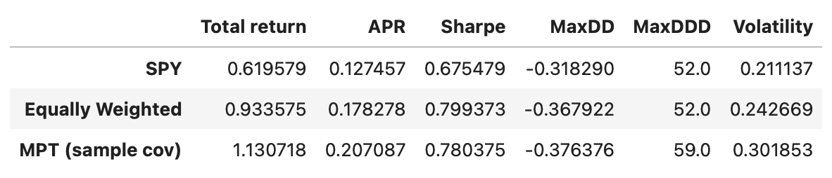
In terms of Sharpe ratios all the strategies have similar performance. Equally weighted portfolio and MPT-based strategy perform a little better; but we have to keep in mind that the transaction costs would be a lot higher, potentially negating any advantage over a simple buy-and-hold SPY strategy.
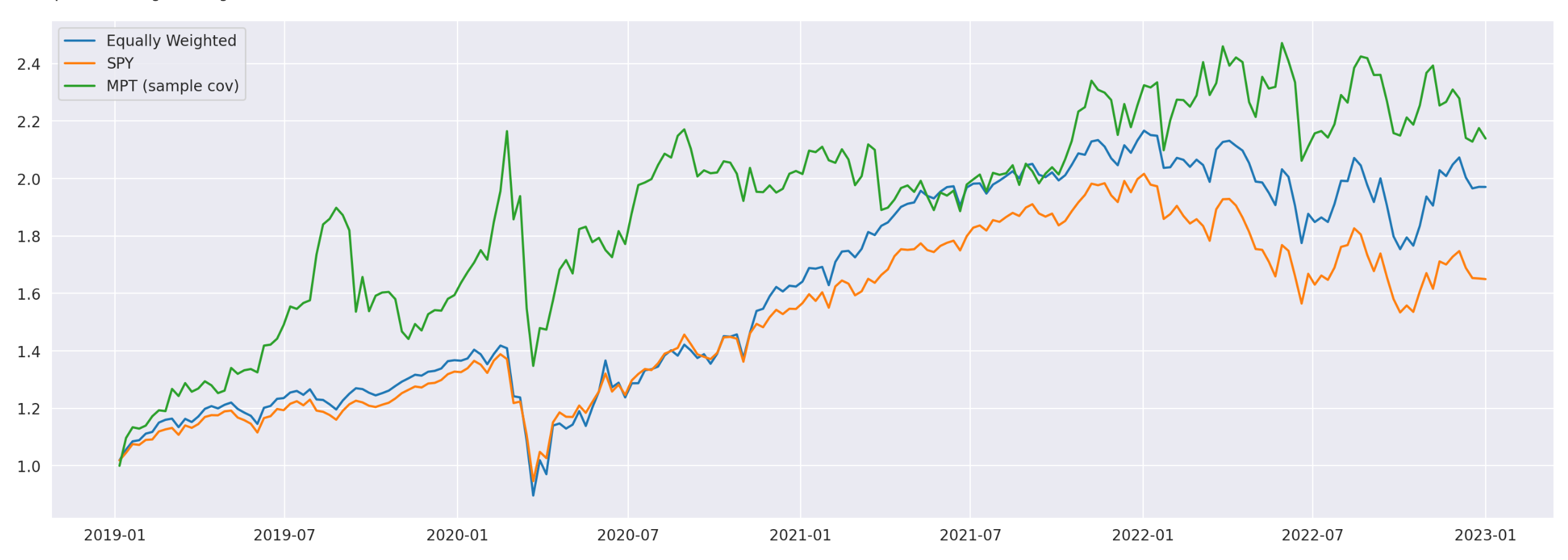
Let’s also plot their cumulative returns to visually assess their performance.
These are all baseline models that we will use for comparison purposes. Now, we can begin to introduce factor models to determine whether they can help improve trading performance.
We start with a simple one-factor model: Single Index Model (SIM), which was developed by William Sharpe in 1963. SIM decomposes returns of a given stock into two components:
A systematic component that is correlated with the overall market movement.
An idiosyncratic component that is specific to the individual stock.
This model assumes that the primary factor affecting a stock's return is its relationship with the broader market. The systematic component is typically represented by the market return, while the idiosyncratic component captures all other factors unique to the stock.
Mathematically it can be described as follows.
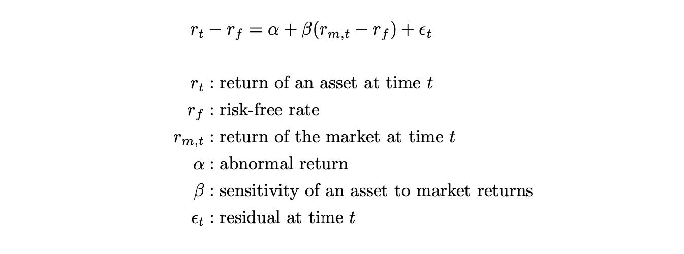
The residuals epsilon represent the portion of asset returns that cannot be explained by other variables. They are assumed to be independent and identically distributed (i.i.d.) Gaussian random variables with zero mean. It is also assumed that the residuals of different assets are uncorrelated.
The model has two parameters (alpha and beta), which can be estimated with OLS (ordinary least squares). Let’s assume for simplicity that risk-free rate is zero. Then for each asset i we have:

To estimate the parameters of the model we can run a set of linear regressions (one for each asset) using the equation above. Then each asset can be described by two numbers - its coefficients, alpha and beta. To calculate the mean and variance of asset returns we can use the following formulas.
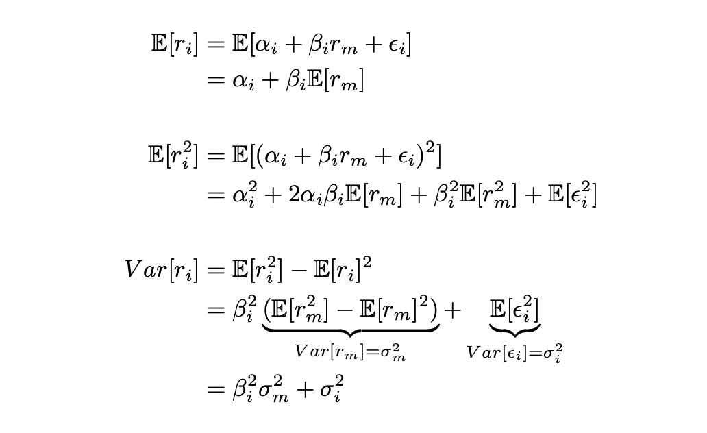
Formula for calculating covariance between the assets can be derived similarly. I’m not going to show the derivation, just the final result.

Covariance now depends only on the volatility of the market and the beta parameter of an asset. Instead of estimating covariance for each pair of stocks individually (124750 covariances for a universe of 500 stocks), we just need to estimate the beta of each stock (500 parameters for 500 stock) and use them to calculate covariances.
In order to estimate covariance matrix of multiple assets, we first use OLS to estimate parameters alpha and beta of each asset, and then apply the following estimators.

We first calculate sample variance of the market and matrix Psi - the diagonal matrix of sample variances of residuals. We then use these estimates to calculate covariance matrix of the assets.
Of course it is important that the factor model we use represents the data reasonably well; otherwise, it won’t be helpful. Therefore I am going to analyse how well the Single-Index Model is able to explain asset returns. In order to do it, I’ll fit the model on each asset individually and save some of its performance metrics in a dataframe.
First we need to prepare the data that we need for this model: return of the market and risk-free return rate. I’m going to use the data from Fama-French factors dataset, which is described later in the article.
| factors_df = pd.read_csv('F-F_Research_Data_Factors_daily.CSV', skiprows=4, index_col=0).iloc[:-1] | |
| factors_df.index = pd.to_datetime(factors_df.index) | |
| factors_df = factors_df.loc[returns.index] # keep only relevant dates | |
| factors_df /= 100 # percentage to decimal | |
| returns_rf = returns - factors_df['RF'].values.reshape(-1,1) # returns minus risk-free rate | |
| mkt_rf = factors_df[['Mkt-RF']] # market return minus risk-free rate |
We are going to work with two dataframes: returns_rf contains returns of the assets minus risk-free rate and mkt_rf contains market returns minus risk-free rate.
| import statsmodels.api as sm | |
| import statsmodels.stats.api as sms | |
| metrics_df = pd.DataFrame(columns=['alpha', 'beta', 'alpha_pval', 'beta_pval', 'R_sq', 'Durbin-Watson', 'JB pval']) | |
| for stock in tqdm(returns_rf.columns): | |
| res = sm.OLS(returns_rf[stock].values, sm.add_constant(mkt_rf.values)).fit() # fit a model | |
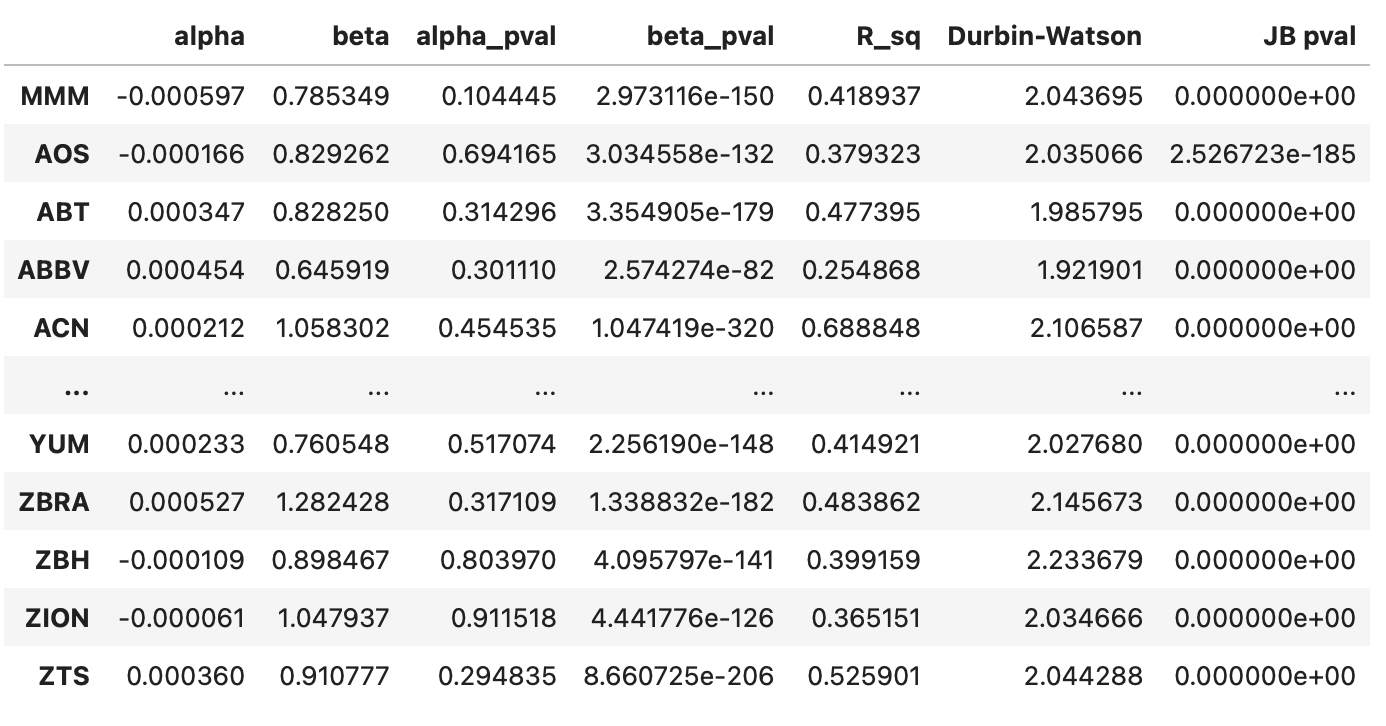
| metrics_df.loc[stock] = [*res.params, *res.pvalues, res.rsquared, sms.durbin_watson(res.resid), sms.jarque_bera(res.resid)[1]] # save metrics |
The resulting dataframe is shown below. For each stock, we have the following columns:
Parameters alpha and beta.
Pvalues for the parameters alpha and beta indicating the probability each parameter is equal to zero.
Coefficient of determination R^2.
Durbin-Watson statistic (should be close to 2 to indicate a lack of autocorrelation in the residuals).
Jarque-Bera pvalue, indicating the probability that the residuals are normally distributed.
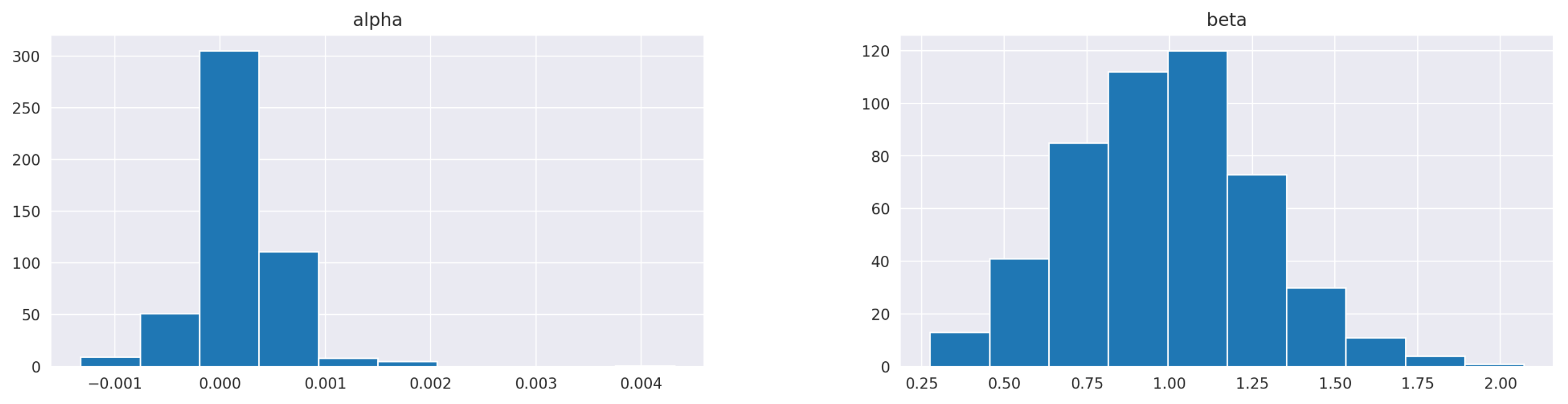
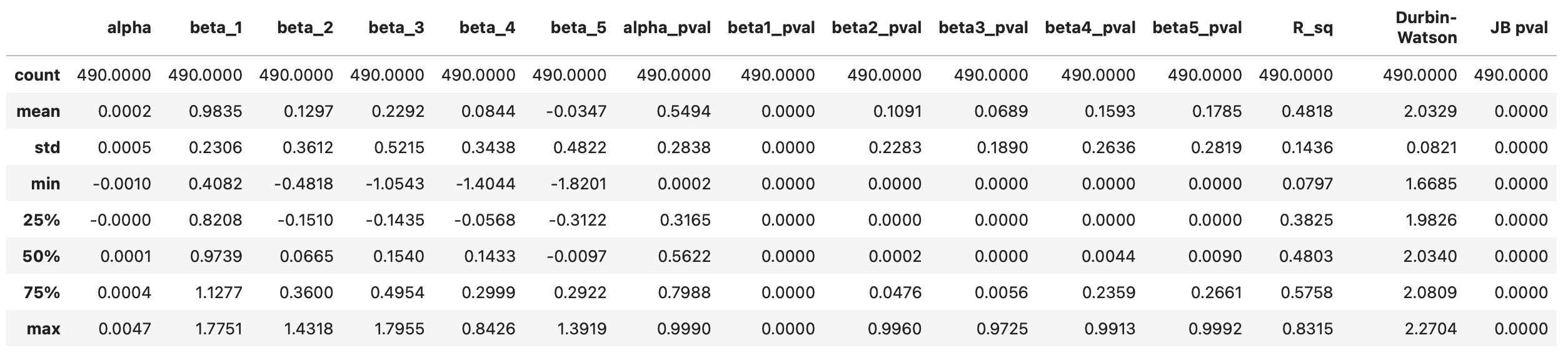
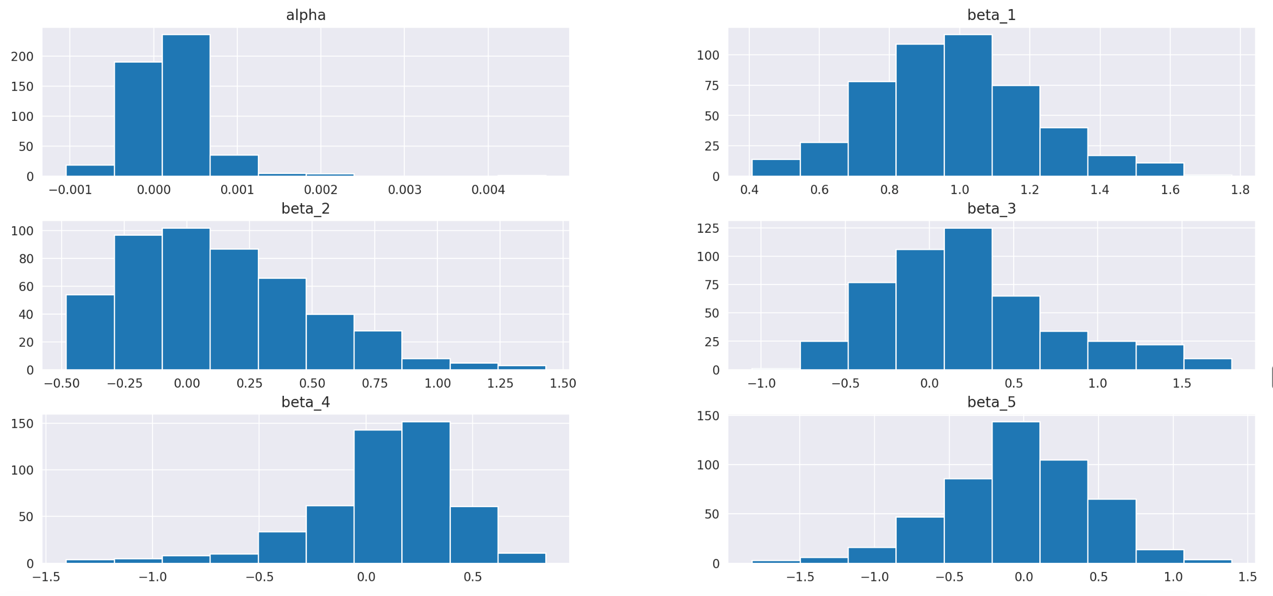
First, let’s take a look at the summary statistics. We can see clearly that parameters alpha are consistently very small and insignificant. Parameters beta, on the other hand, range from 0.27 to 2.07 and are never close to zero. This can also be observed on the histogram shown below the table.
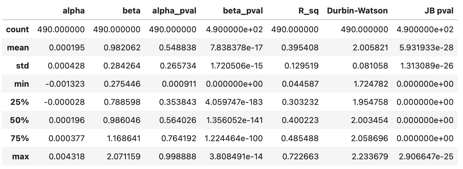
Another thing we can notice is that pvalues of Jarque-Bera test are always very close to zero. That means that it’s very unlikely that the residuals are normally distributed, which in turn suggests that our model is not very effective at explaining the data.
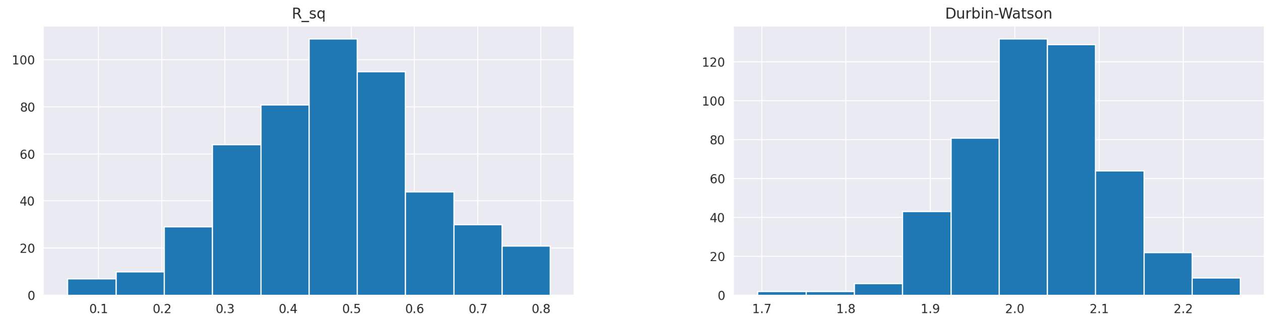
Finally, let’s look at the histograms of R-squared values and Durbin-Watson statistics.
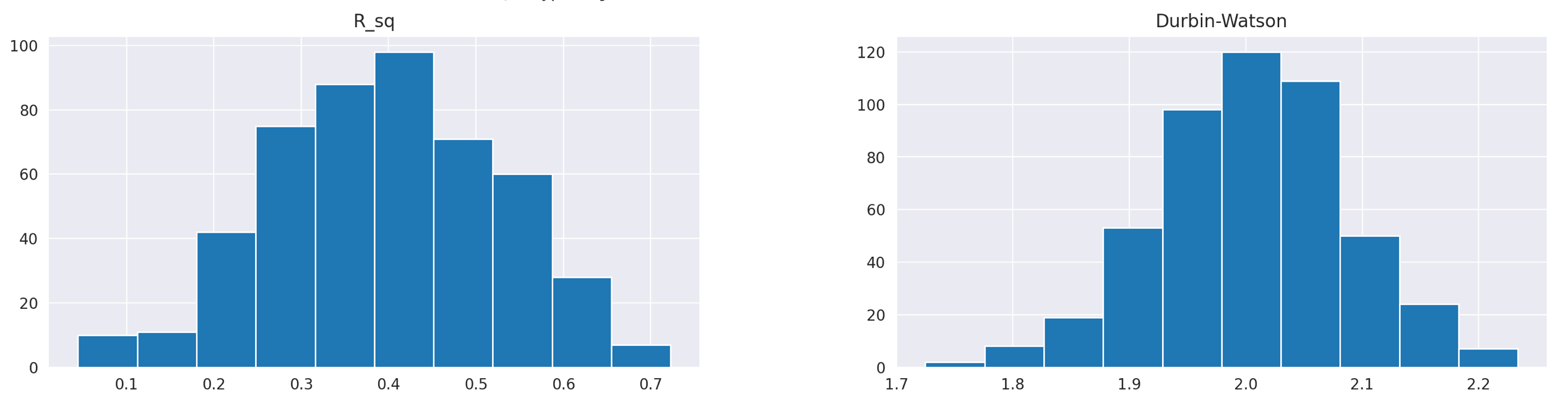
R squared values are centered around 0.4, meaning that, on average, our regression model explains 40% of variability in the target variable. The Durbin-Watson statistic ranges from 1.7 to 2.2 and is centred around 2, which is a good sign, indicating no autocorrelation in residuals.
To summarise, the single-index model is not very effective, but it demonstrates that market returns have a significant impact on the returns of all assets. Let’s try to incorporate it in our strategy.
The code for backtesting this strategy is almost identical to the previous one. The only difference is the way we calculate covariance matrix, which is used as an input for the optimization problem. Lines 17-18 in the code below are used to fit the model and save the beta parameters in a dataframe. Lines 22-24 are used to calculate the covariance matrix. Note that when calculating variances and covariances, we must account for the degrees of freedom, which depend on the number of factors in the model. To do this, we adjust the ddof parameter in np.cov and np.var functions.
| from sklearn.linear_model import LinearRegression | |
| positions = pd.DataFrame(index=returns_w.loc['2019-01-01':].index, columns=returns_w.columns) | |
| target_vol = volatility_eqw | |
| bounds=[[0,1]]*len(stocks) | |
| x0 = np.ones(len(stocks)) / len(stocks) | |
| for t in tqdm(returns_w.loc['2019-01-01':].index): | |
| # prepare data | |
| prices_tmp = prices.loc[:t].iloc[-252:] | |
| returns_tmp = prices_tmp.pct_change().dropna() | |
| returns_rf_tmp = returns_rf.loc[returns_tmp.index] | |
| mkt_tmp = mkt_rf.loc[returns_tmp.index] | |
| # fit factor model | |
| res = LinearRegression().fit(mkt_tmp.values, returns_rf_tmp.values) | |
| betas = pd.DataFrame(res.coef_.flatten(), index=returns.columns, columns=['Beta']) | |
| # calculate covariance | |
| # use ddof in np.var and np.cov to account for a number of factors | |
| resid = returns_rf_tmp.values - res.predict(mkt_tmp.values) # residuals | |
| psi = np.diag(np.diag(np.cov(resid.T, ddof=2))) # residuals variance | |
| cov_factor = betas.values @ betas.values.T * mkt_tmp.values.var(ddof=1) + psi | |
| # perform optimization | |
| constraints = ({'type':'eq', 'fun': lambda x: volatility(x,cov_factor)-target_vol}, | |
| {'type':'eq', 'fun': lambda x: np.sum(x)-1}) | |
| res = minimize(negative_annual_return, x0, args=(returns_rf_tmp.mean()), | |
| bounds=bounds, constraints=constraints) | |
| if res.status!=0: | |
| print('Optimization failed') | |
| positions.loc[t] = positions.loc[:t].iloc[-2] # keep previous weights | |
| else: | |
| positions.loc[t] = res.x |
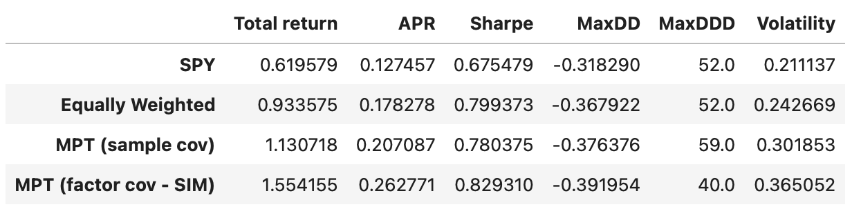
This strategy performs a little better than the previous ones, but it has higher drawdown and volatility. However, it achieves an APR of 26%, and maximum drawdown duration is reduced by nearly 20 weeks, compared to the strategy with sample covariance matrix. Let’s see if we can improve it with other factor models.
Now we are going to consider Fama-French 3-factor and 5-factor models, but first let me introduce a little bit of math and show how to generalize one-factor model we used above to account for any number of factors. For simplicity, I will assume that the risk-free rate is zero.
Suppose we have K factors. Then return of a given asset at time t can be expressed as follows.

Factors f_1 to f_K are the same for each asset, but vary over time. Parameters alpha and beta_1 to beta_K are specific to each asset, but remain constant over time. Epsilon represents the asset-specific idiosyncratic component. Parameter alpha is called the intercept, while parameters beta_1 - beta_K are called factor loadings.
Returns of a given asset over time range from 1 to T can be expressed as follows.

Or, alternatively, it can be written in matrix form like this:

Using the equation above and performing a linear regression we can estimate parameters alpha and beta for a given asset.
Below I demonstrate how to combine all the assets and all time periods in matrix form. I assume there are m assets, K factors, and T time periods.
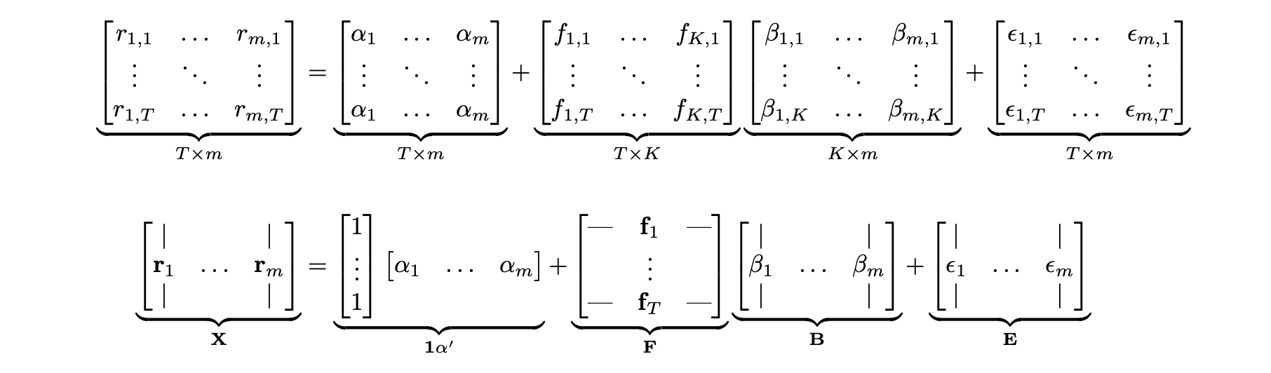
The two lines above show different representations of the same equation. In the first line, each variable is shown explicitly, allowing us to check that the dimensions of all matrices match. The second line represents each matrix as a collection of column or row vectors. Matrix X consists of m column vectors of returns (one for each asset). Matrix F consists of T column vectors of factors - one vector of factor realisations for each time period. Matrix B consists of m column vectors of factor loadings (with K factor loadings for each of the m assets). Finally, matrix E consists of m column vectors of residuals.
Combining it all together we get the following matrix equation.

This approach allows us to perform a single multivariate regression instead of running a separate regression for each asset (which is especially important if we aim to trade at higher frequencies or with a larger universe of assets).
After running the multivariate regression and estimating the parameter matrix B, we can calculate the covariance matrix of returns. First we need to estimate the following parameters.
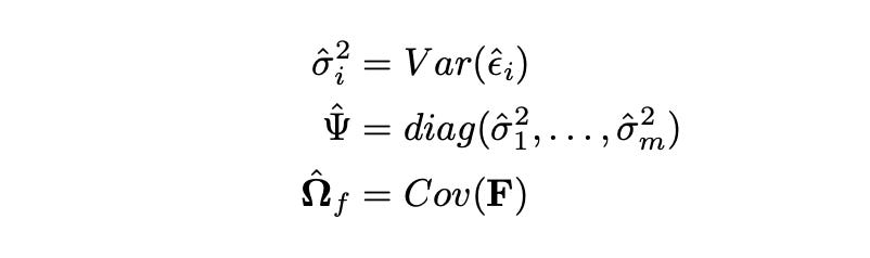
Matrix Psi above is the diagonal matrix of sample variances of residuals, and matrix Omega_f is the sample covariance matrix of the factor returns.
Using the parameters outlined above, we can now calculate the covariance matrix.

We can apply this procedure to models with any number of factors. While the equations might seem complex, it will be easy to apply them in practice.
The first multi-factor model we are going to test is Fama-French three-factor model. It is one of the most famous and widely used factor models in finance, developed in 1992 by Nobel laureates Eugene Fama and Kenneth French. In addition to the market return, used in the previous model, this model incorporates two more factors: SMB and HML. SMB stands for ‘Small Minus Big’ and represents the difference of returns between small-cap and large-cap stocks. HML stands for ‘High Minus Low’ and represents the difference of returns between high book-to-market stocks and low book-to-value stocks.
The final formula is shown below.

Now, we can estimate covariance matrix of returns using the formulas for multi-factor models provided above. Let’s give it a try.
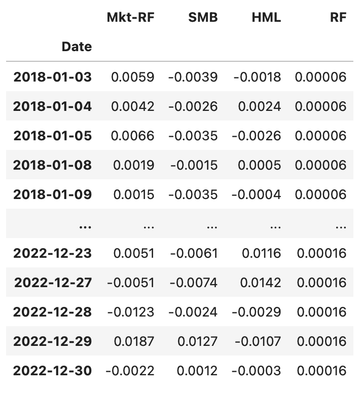
We begin by downloading and preparing the factor data. I am going to use data from Kenneth R. French data library. You can find the description of the specific dataset I’m using here.
| factors_df = pd.read_csv('F-F_Research_Data_Factors_daily.CSV', skiprows=4, index_col=0).iloc[:-1] | |
| factors_df.index = pd.to_datetime(factors_df.index) | |
| factors_df = factors_df.loc[returns.index] # keep only relevant dates | |
| factors_df /= 100 # percentage to decimal |
The resulting dataframe is shown below. The first three columns contain the three factors and the last column contains the risk-free rate for each time period.
Let’s start by assessing the quality of the model. As before, I fit the model on each asset and save performance metrics in a dataframe. Instead of one parameter beta in single-index model, we now have three.
| metrics_df = pd.DataFrame(columns=['alpha', 'beta_1', 'beta_2', 'beta_3', 'alpha_pval', 'beta1_pval', 'beta2_pval', 'beta3_pval', | |
| 'R_sq', 'Durbin-Watson', 'JB pval']) | |
| for stock in tqdm(returns_rf.columns): | |
| res = sm.OLS(returns_rf[stock].values, sm.add_constant(factors_df.iloc[:,:3].values)).fit() # fit a model | |
| metrics_df.loc[stock] = [*res.params, *res.pvalues, res.rsquared, sms.durbin_watson(res.resid), sms.jarque_bera(res.resid)[1]] # save metrics |
Summary statistics of the resulting dataframe are shown below. Again, we can see that the intercept alpha is always insignificant, while beta_1 is always significant. Coefficients beta_2 and beta_3 seem to be significant, but not in all cases. Histograms of the parameters are also provided below.
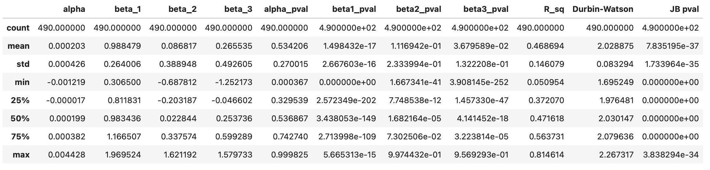
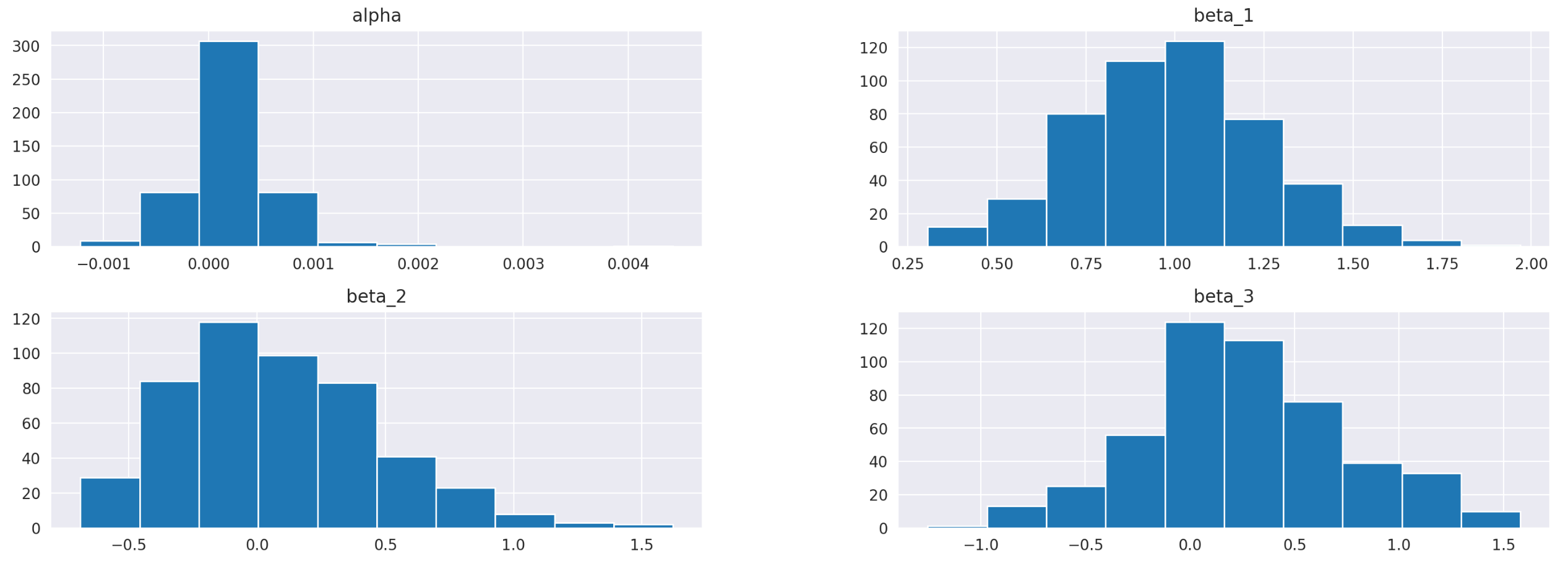
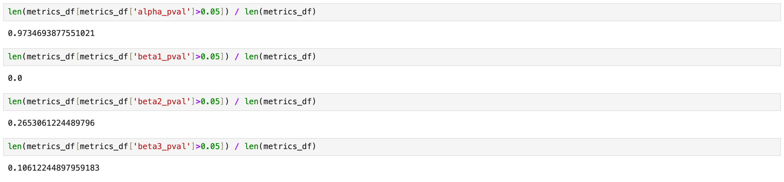
On the screenshot below I’m testing what percentage of assets has more than a 5% probability that a given parameter is zero. Results for parameters alpha and beta_1 are the same as before - alpha is always insignificant, beta_1 is always significant. Parameters beta_2 and beta_3 are less stable. For 26% of the assets, beta_2 may be zero, and for 10% of the assets, beta_3 may be zero.
Finally let’s look at the plots of R^2 and Durbin-Watson statistic. They look very similar to what we obtained previously. However, if we take a closer look at R^2 and check the summary statistics table, we will notice that both the mean and median of R^2 have increased from 0.4 to 0.46. Therefore, adding more parameters to the model has provided a bit more explanatory power. Let’s see how this affects trading performance.
Here we need to introduce a few more changes in the process of calculating the covariance matrix. However, this version will work for any number of factors with only minor adjustments. We fit the linear regression model and then use the parameter estimates along with the formulas provided above to calculate the covariance matrix of the assets.
| positions = pd.DataFrame(index=returns_w.loc['2019-01-01':].index, columns=returns_w.columns) | |
| target_vol = volatility_eqw | |
| bounds=[[0,1]]*len(stocks) | |
| x0 = np.ones(len(stocks)) / len(stocks) | |
| K = 3 # number of factors | |
| for t in tqdm(returns_w.loc['2019-01-01':].index): | |
| # prepare data | |
| prices_tmp = prices.loc[:t].iloc[-252:] | |
| returns_tmp = prices_tmp.pct_change().dropna() | |
| factors_tmp = factors_df.loc[returns_tmp.index] | |
| returns_rf_tmp = returns_rf.loc[returns_tmp.index] | |
| # fit factor model | |
| res = LinearRegression().fit(factors_tmp.iloc[:,:3].values, returns_rf_tmp.values) | |
| B = res.coef_ | |
| # estimate covariance and other parameters | |
| omega_f = factors_tmp.iloc[:,:3].cov() # covariance of the factors | |
| resid = returns_rf_tmp.values - res.predict(factors_tmp.iloc[:,:3].values) # model residuals | |
| psi = np.diag(np.diag(np.cov(resid.T, ddof=K+1))) # residuals variance | |
| cov_factor = B @ omega_f.values @ B.T + psi # covariance of asset returns | |
| # perform optimization | |
| constraints = ({'type':'eq', 'fun': lambda x: volatility(x,cov_factor)-target_vol}, | |
| {'type':'eq', 'fun': lambda x: np.sum(x)-1}) | |
| res = minimize(negative_annual_return, x0, args=(returns_rf_tmp.mean()), | |
| bounds=bounds, constraints=constraints) | |
| if res.status!=0: | |
| print('Optimization failed') | |
| positions.loc[t] = positions.loc[:t].iloc[-2] # keep previous weights | |
| else: | |
| positions.loc[t] = res.x | |
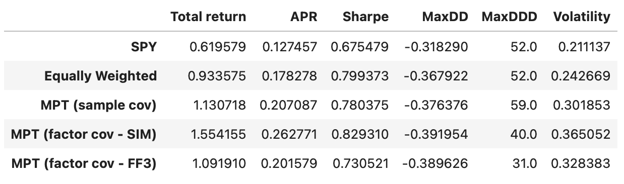
Total return and Sharpe ratio decrease slightly, but at the same time, we are moving closer to the target volatility of 24%. Both maximum drawdown and maximum drawdown duration also decrease. Recall that our optimization objective is to maximize return for a given level of volatility, and this model helps us get a bit closer to that objective. It would be interesting to see what happens if we optimize for maximum Sharpe ratio, but that will be a topic for another article.
Now, let’s move to Fama-French five-factor model. A description of the factor dataset I’m using can be found here. Everything we do here is similar to the previous section, so I’m going to skip the explanations and just provide the results.
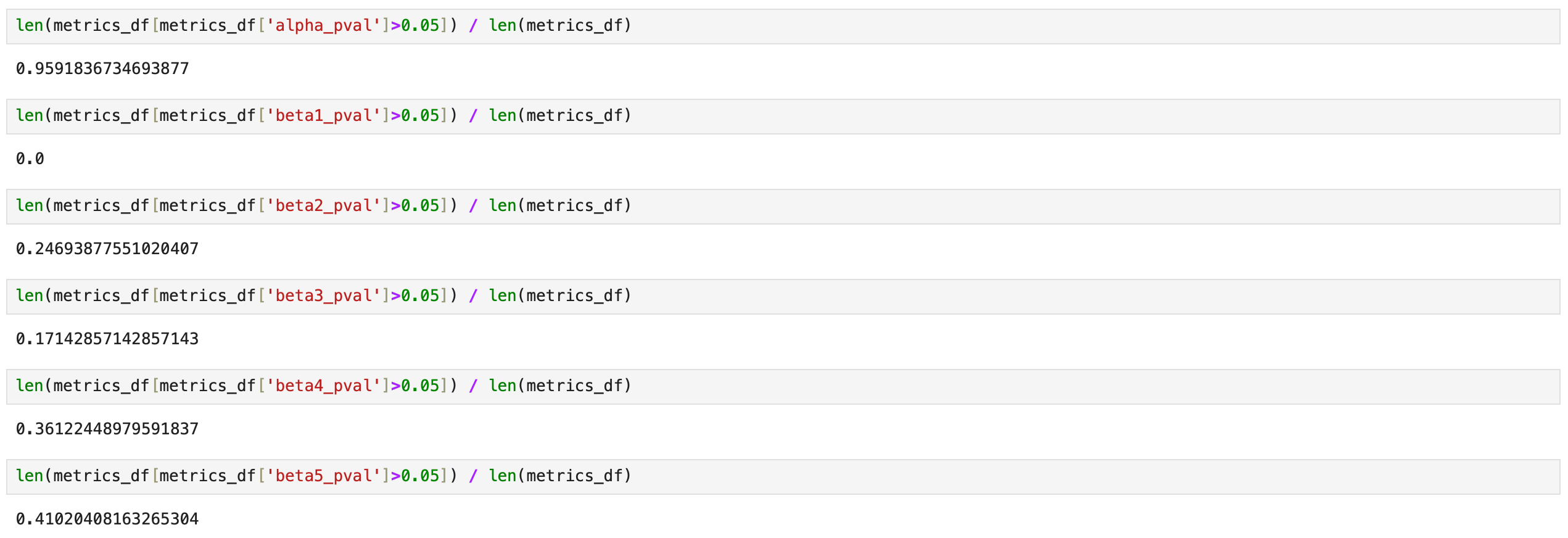
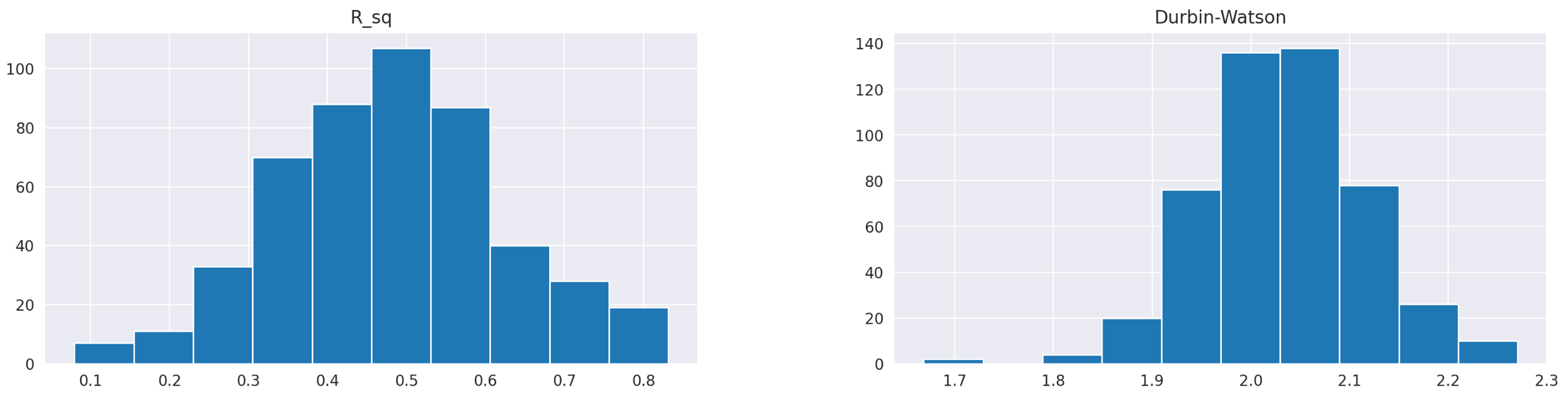
The R^2 value increased only slightly, from 47% to 48%. Additionally, the parameters beta_4 and beta_5 may be zero for a larger percentage of assets. Overall, the findings are similar to those of the three-factor model. We may not see any increase in trading performance, but let’s find out.
| positions = pd.DataFrame(index=returns_w.loc['2019-01-01':].index, columns=returns_w.columns) | |
| target_vol = volatility_eqw | |
| bounds=[[0,1]]*len(stocks) | |
| x0 = np.ones(len(stocks)) / len(stocks) | |
| K = 5 # number of factors | |
| for t in tqdm(returns_w.loc['2019-01-01':].index): | |
| # prepare data | |
| prices_tmp = prices.loc[:t].iloc[-252:] | |
| returns_tmp = prices_tmp.pct_change().dropna() | |
| factors_tmp = factors_df.loc[returns_tmp.index] | |
| returns_rf_tmp = returns_rf.loc[returns_tmp.index] | |
| # fit factor model | |
| res = LinearRegression().fit(factors_tmp.iloc[:,:5].values, returns_rf_tmp.values) | |
| B = res.coef_ | |
| # estimate covariance and other parameters | |
| omega_f = factors_tmp.iloc[:,:5].cov() # covariance of the factors | |
| resid = returns_rf_tmp.values - res.predict(factors_tmp.iloc[:,:5].values) # model residuals | |
| psi = np.diag(np.diag(np.cov(resid.T, ddof=K+1))) # residuals variance | |
| cov_factor = B @ omega_f.values @ B.T + psi # covariance of asset returns | |
| # perform optimization | |
| constraints = ({'type':'eq', 'fun': lambda x: volatility(x,cov_factor)-target_vol}, | |
| {'type':'eq', 'fun': lambda x: np.sum(x)-1}) | |
| res = minimize(negative_annual_return, x0, args=(returns_rf_tmp.mean()), | |
| bounds=bounds, constraints=constraints) | |
| if res.status!=0: | |
| print('Optimization failed') | |
| positions.loc[t] = positions.loc[:t].iloc[-2] # keep previous weights | |
| else: | |
| positions.loc[t] = res.x |
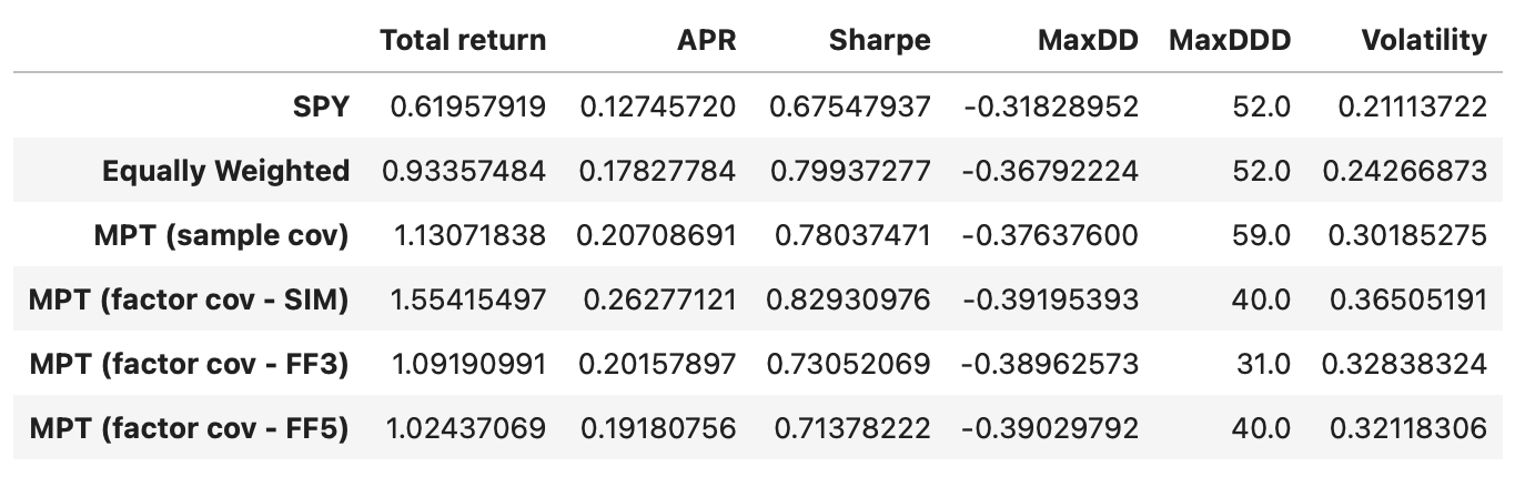
Performance metrics of the strategy using 5-factor model are not higher compared to the strategy using 3-factor model. In fact they are a little lower. This is not surprising considering that both models are very similar in terms of the data variability that they explain.
The performance metrics of the strategy using the FF5 model are not higher compared to those using the FF3 model; in fact, they are slightly lower. This is not surprising, given that both models are very similar in terms of the data variability they explain.
Let’s take a look at the cumulative returns of all the strategies tested so far.
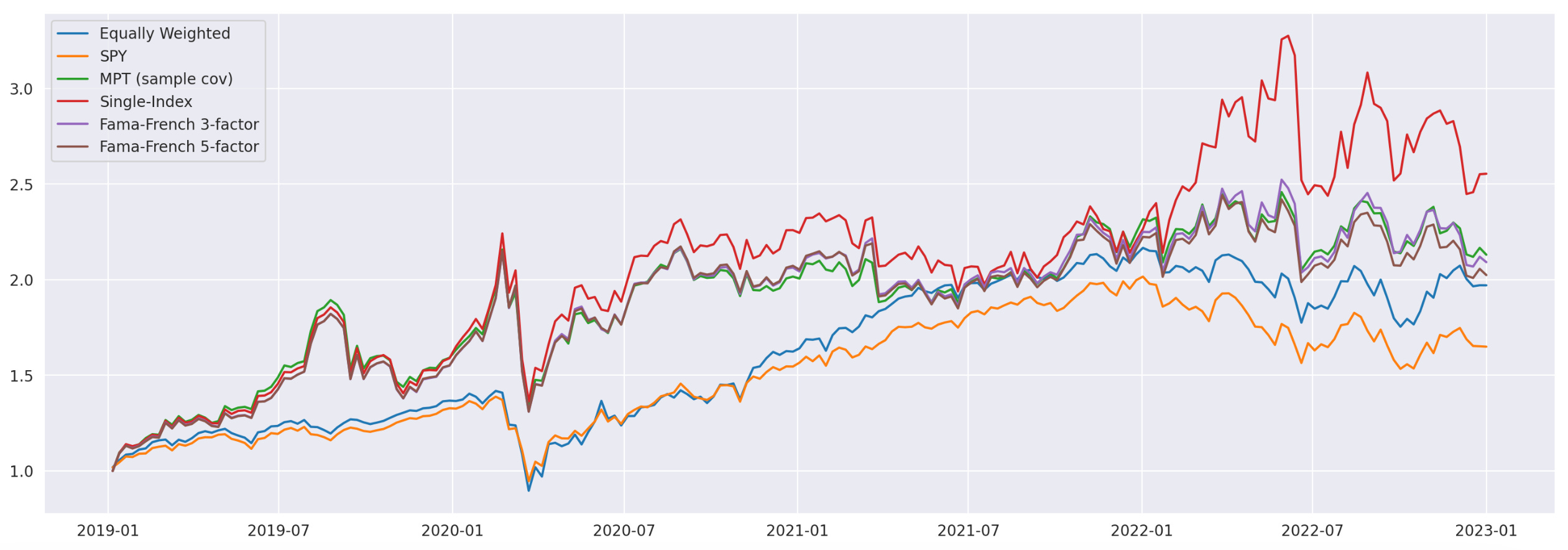
The strategies based on the Fama-French 3-factor (FF3) and 5-factor (FF5) models exhibit nearly identical cumulative returns, indicating that using the FF5 model in this particular strategy does not provide any added value.
While the single-index model demonstrates the highest total return among all the tested strategies, it also carries the most risk. On the other hand, the strategy based on the sample covariance matrix achieved a volatility level closest to the target level of 24% (volatility of the equally weighted portfolio). As of now, it remains unclear whether the factor models tested offer any trading advantages; it’s possible that the models may not be as effective as anticipated.
This article has turned out longer than I expected, so I will pause here and continue in a second part, where I will explore how to use Principal Component Analysis (PCA) to derive our own factors from the data, rather than relying solely on traditional factors from Fama-French and other models. I will also compare the performance of trading strategies based on PCA-derived factors to those tested here.
Keep in mind that estimating the covariance matrix is just one basic use case of factor models. There are numerous other applications, far too many to cover in a single article — or even in an entire book.
Jupyter notebook with source code is available here.
If you have any questions, suggestions or corrections please post them in the comments. Thanks for reading.
References
[2] https://youtube.com/watch?v=ro07evEWbCE
[3] https://en.wikipedia.org/wiki/Single-index_model
[4] Introduction to Portfolio Optimization and Modern Portfolio Theory
[5] Portfolio Optimization with Weighted Mean and Covariance Estimators
[6] Quantitative Equity Investing (Fabozzi et al. 2010)
[7] https://statisticsbyjim.com/hypothesis-testing/degrees-freedom-statistics/