Pricing derivatives with binomial tree model (Part 2)
A step-by-step guide to basic binomial option pricing.
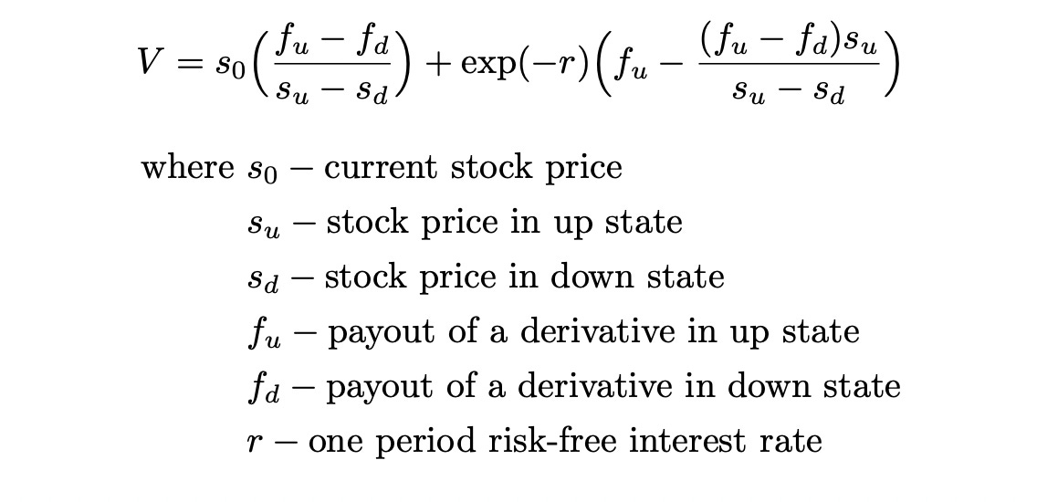
In the previous article we discussed several simple examples to get a general intuition behind binomial tree pricing model. Now I want to describe that model in a little bit more abstract mathematical terms. Recall that we got a formula that can be used to price any derivative in 1-period binomial model. We also discussed why we need to use no-arbitrage principle and price derivative contracts by constructing a portfolio that replicates the payout of derivate in each state of the world. The formula is shown below.
The formula above does not include actual probabilities of being in up or down states. Recall also that in numerical examples in the previous article we found out that using actual probabilities to calculate expected value of the stock and using it to price derivatives led to arbitrage.
Let’s define a quantity q as follows:
If q is less than 0 then we have an arbitrage opportunity: borrow s_0, buy a stock and in any state of the world get a rate of return bigger than r. If q is greater than one, there is again an arbitrage opportunity: short sell a stock for s_0, invest the money it at risk-free rate r, get a positive profit at the end of the period after buying and returning the stock. From this we can conclude that if there is no arbitrage opportunities, q must be between 0 and 1. Now let’s think of q as a probability (we can do this because it belongs to an interval [0,1]). If we thank of q as a probability then we can define expected value of the discounted derivative payout as follows:
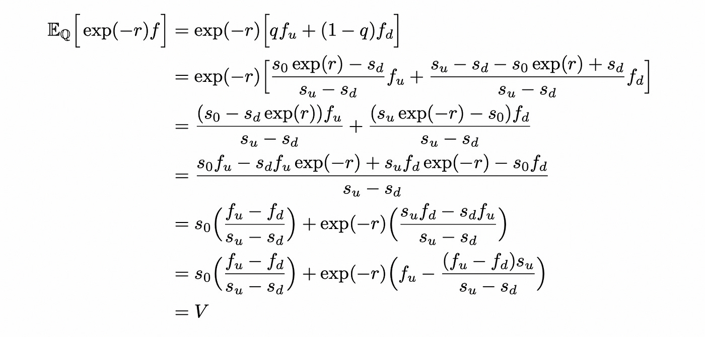
The subscript Q of the expectation indicates that we are using probabilities q. Now let’s look at this formula a little closer.
So, using a little bit of algebra we were able to express the price of derivative (equal to the price of replicating portfolio) as an expectation of the discounted derivative payout. But expectation not under true probabilities Pof being in up or down states, but under synthetic probabilities Q. Right now it doesn’t seem useful — we just rewrote the same formula in a different terms, but it will be helpful later.
To proceed further we need to introduce some terminology and formally define different parts of the model.
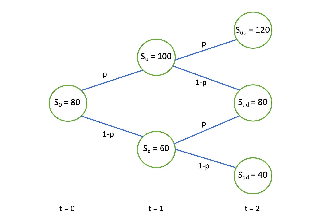
Process S is a set of all possible stock values and their connections to each other. It can be represented as a graph shown below. Assume that the subscript of S indicates the ‘name’ of the node.
Random variable S_i is a value of the process S at a particular time (for example at time t=1, S_1 is either S_u or S_d).
Probability measure is a set of probabilities used (p and (1-p) in the example above).
Filtration F_i is a history of the process up to the time t=i (if at time t=2the process is in state uu then F_2 = {0, u, uu}).
Claim X with time-horizon T is a function of filtration F_T. For simple put and call option it will just be a function of the current stock price at time t=T. For some other derivatives it may depend on previous states (for example, the maximum price the stock reached up to time t=T).
Previsible process is a process on the same graph whose value at time t=iis known at time t=i-1 (it depends only on filtration F_{i-1}).
Martingale is a stochastic process for which the conditional expected value (given observations up to time t=i) at time t≥i+1 is equal to the value of the process at time t=i. More formally we can call it a martingale with respect to probability measure P given filtration F_i.
Now we are ready to state the binomial representation theorem.
Binomial representation theorem:
Let S be a binomial price process and Q be probability measure under which the process S is a martingale. Then for any other Q-martingale N there exists a previsible process phi, such that
Delta_S indicates the change in the stock price from time t=k-1 to time t=k. The formula above means that we can express the change in N as change in Sscaled by phi.
In the next section I describe how to find that phi and show why binomial representation theorem is true. Feel free to skip it if you are not interested in underlying math. I will provide a formula for phi in the section describing financial application.
Assume that we are at time t=0 and we want to find such phi. Let Z be an indicator random variable that shows whether we are in up or down state at time t=1.
We have:
Define new quantity Phi:
Multiply delta_S_1 by Phi:
Now let’s try to express delta_N_1 in terms of delta_S_1. We just add missing terms and subtract terms that we don’t need:
The calculations above show that we can express change in N as change in Sscaled by Phi and shifted by ksi.
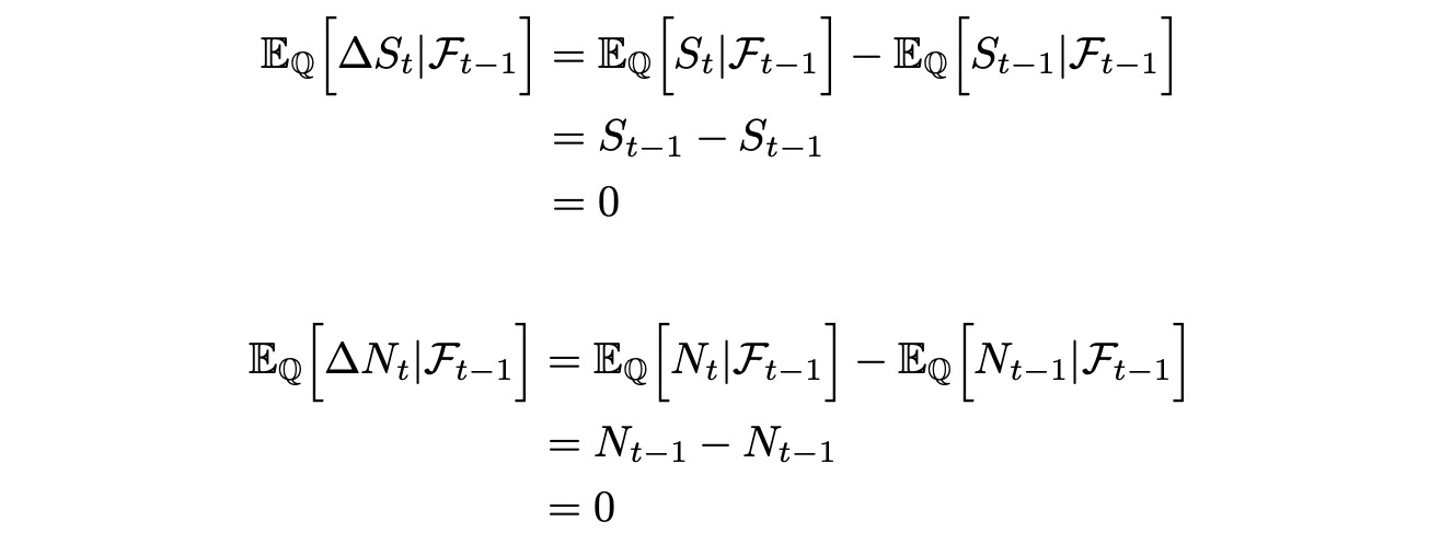
Since S and N are Q-martingales we have:
Express expected value of delta_N as expected value of scaled and shifted delta_S:
In the last line above we can take Phi and ksi out of expectation because they are known beforehand (not random). We also know that the expected values of delta_N and delta_S are zero (as shown above). Then:
For the expression above to be equal to zero, ksi must be zero. From this we can conclude that change in N can be expressed as scaled change in S.
Now let’s see how it applies to pricing derivatives. Assume we have a bond process B_i, which we use to track the time-value of money. It is positive and previsible (since we assume that return of the bond is the same in any state of the world) and B_0=1. Also define:
For the next step we need Z_i to be a martingale with respect to some probability measure Q. Let’s check if it is true. I will demonstrate why it is true for the first time interval. The calculation is the same for all other cases. We need to show that:
Rewriting:
Solving for q:
If such q exists and lies in the interval between 0 and 1, then there is a probability measure Q under which the discounted stock process Z is a martingale. But this is the same expression we had in the beginning of the article and we’ve already shown that it lies in the interval [0,1].
Now we can safely assume that discounted stock process Z is a Q-martingale. Assume we have a claim X. Then we can define process E_i as follows:
So E_i is defined as expected value (under Q) of the discounted claim at time t=i given filtration F_i. We can show that process E is Q-martingale.
Above we show that the expected value of E (under Q) at time t=j given filtration F_i is equal to the current value of E (at time t=i). That means that process E is Q-martingale.
Now we have two processes — discounted stock process Z and discounted claim process X, which are both Q-martingales. Then from binomial representation theorem we can infer that there exists previsible process phi such that:
That means that expected value of discounted claim is previsible. Therefore we can construct a portfolio (one time step before) which will be worth the expected value of discounted claim at the next time step (regardless of whether the stock moves up or down).
At time t=0 we construct a portfolio which is equal to the expected value (under Q) of discounted claim:
Phi_1 is the number of stocks to buy and psi_1 is the amount of cash to invest at risk-free rate (in bonds). We know that process phi is previsible, so phi_1 is known at time t=0. Formula for calculating it is shown below (see the previous section for detailed explanation).
Expected value of the discounted claim E_0 is also known. Then psi_1 can be calculated as follows:
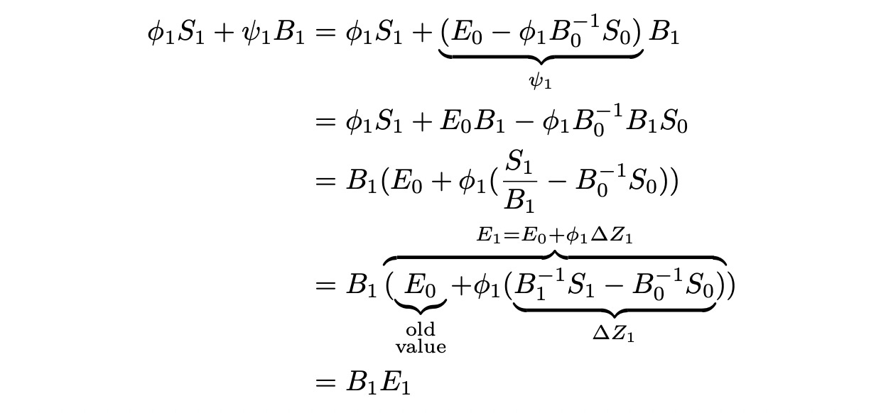
What happens in the end of the period? The value of portfolio changes, it is now worth:
At time t=1 we need to construct another portfolio — phi_2 stocks and psi_2bonds. Let’s calculate how much it costs.
This new portfolio has exactly the same value as our previous portfolio. So we can sell the previous portfolio and buy the new portfolio without any additional investments. All the next steps are calculated in the same way. Each time after selling the portfolio from the previous time step we will get precisely the amount required to buy another portfolio and proceed to the next time step. At time T (maturity of the claim X) we have the following portfolio:
So we have shown that starting with a certain portfolio (of stock and bond) at time t=0 we can create a self-financing (not requiring additional investments) strategy that replicates the payout of a given claim X at time t=T. Price of such portfolio is equal to the expected value of discounted claim under martingale measure Q. By no-arbitrage principle this is the only price which doesn’t allow arbitrage. If the price was different, someone could buy\sell derivative and then run the strategy to replicate it’s payout and make riskless profit.
Now let’s implement binomial pricing model in Python. The only thing we didn't discuss yet is how to determine the price of the stock in up and down states. It can be determined from the volatility of log prices of the stock as follows:
The stock price is calculated by multiplying the stock price at the previous state by either u or d depending on the state.
We also need to calculate probabilities of up and down moves under which the discounted stock process is a martingale. These probabilities are also called risk-neutral probabilities. We can use the same formulas as before:
Assume we want to calculate the price of European call and put options with maturity at time t=T. European options can be executed only at time T, so their payout depend only on the stock price at time T. What we need to do then is to calculate stock prices and corresponding probabilities for all possible states at time T. It is done using binomial tree with a given number of periods. Using this information we can calculate the price of an option which is equal to the expected value of discounted option payout under risk-neutral probabilities.
We are going to use the following parameters:
| N = 2 # number of periods | |
| T = 1 # total time (in years) | |
| S_0 = 50 # initial stock price | |
| K = 60 # option strike price | |
| dt = T/N # delta t | |
| sigma = 0.4 # annual stock volatility | |
| r = 0.05 # annual risk free rate |
We want to price an option with strike price K=60 maturing in T=1 year. Current stock price S_0=50, annual stock volatility sigma=0.4 and annual risk-free rate r=0.05. At first we will use N=2 steps, so that we can easily check the results by hand.
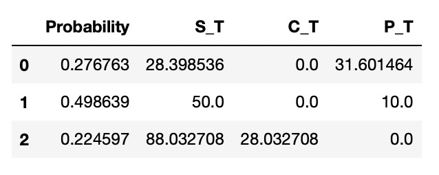
First we calculate value of up and down moves — u and d, and risk-neutral probability p. Then we find the price of the stock in all possible terminal states and probability of each state (it’s basically a binomial distribution). Using the stock price we also calculate the value (at maturity) of call and put options. Results are saved to a dataframe.
| u = np.exp(sigma * np.sqrt(dt)) # up move | |
| d = np.exp(-sigma * np.sqrt(dt)) # down move | |
| p = (np.exp(r*dt) - d) / (u - d) # risk-neutral probability | |
| df = pd.DataFrame(index=np.arange(N+1), columns=['Probability', 'S_T', 'C_T', 'P_T']) | |
| for i in range(N+1): | |
| S_T = S_0 * u**i * d**(N-i) # stock prices at time T | |
| prob = comb(N,i) * p**i * (1-p)**(N-i) # probability of ending up at state with stock price S_T | |
| C_T = np.max([S_T-K,0]) # value of a call option at T | |
| P_T = np.max([K-S_T,0]) # value of a put option at T | |
| df.loc[i] = [prob, S_T, C_T, P_T] |
Look at the resulting dataframe below.
We can check that the calculated probabilities and prices are correct. On the screenshot below we check that the price of the stock after two up moves is 88.03 and probability of two up moves is 0.2246. This matches the results we have in a dataframe.
To calculate the price of an option we need to find the expected value of its discounted payout under risk-neutral (martingale) probabilities.
| C = (df['Probability'] * df['C_T']).sum() * np.exp(-r*T) # discounted expectation of call value | |
| P = (df['Probability'] * df['P_T']).sum() * np.exp(-r*T) # discounted expectation of put value |
We get the following prices:
Below you can find the same code packed in a function.
| def binomial_price(S_0, K, T, N, sigma, r): | |
| ''' | |
| calculate price of call and put option on stock S | |
| Args: | |
| S_0 (float): current stock price | |
| K (float): option strike price | |
| T (float): time to option maturity (in years) | |
| N (integer): number of time steps to use | |
| sigma (float): annual volatility of stock log prices | |
| r (float): annual risk-free rate | |
| Returns: | |
| C (float): price of call option | |
| P (float): price of put option | |
| ''' | |
| dt = T/N # delta t | |
| u = np.exp(sigma * np.sqrt(dt)) # up move | |
| d = np.exp(-sigma * np.sqrt(dt)) # down move | |
| p = (np.exp(r*dt) - d) / (u - d) # risk-free probability | |
| df = pd.DataFrame(index=np.arange(N+1), columns=['Probability', 'S_T', 'C_T', 'P_T']) | |
| for i in range(N+1): | |
| S_T = S_0 * u**i * d**(N-i) # stock prices at time T | |
| prob = comb(N,i) * p**i * (1-p)**(N-i) # probability of ending up at state with stock price S_T | |
| C_T = np.max([S_T-K,0]) # value of a call option at T | |
| P_T = np.max([K-S_T,0]) # value of a put option at T | |
| df.loc[i] = [prob, S_T, C_T, P_T] | |
| C = (df['Probability'] * df['C_T']).sum() * np.exp(-r*T) # discounted expectation of call value | |
| P = (df['Probability'] * df['P_T']).sum() * np.exp(-r*T) # discounted expectation of put value | |
| return C,P |
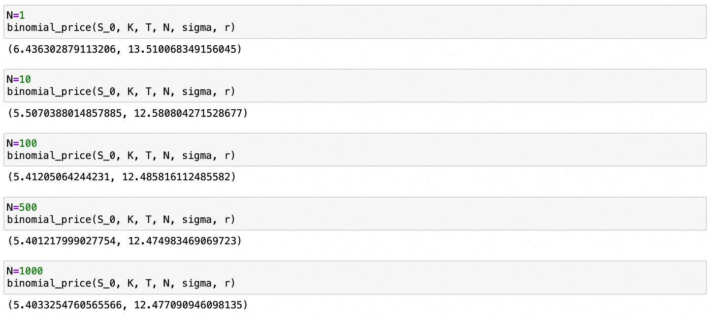
Let’s see how the number of intervals affect the resulting price. On the screenshot below you can see the results of my experiment with different number of intervals N.
After N=100 we get only tiny changes in option prices. We can compare our results to the results of Black-Scholes pricing model. I used Black-Scholes model calculator available here.
Starting with a very simple binomial model we were able to get very good results. With high enough number of time periods N our results match those of the Black-Scholes model.
Jupyter notebook with source code is available here.
If you have any questions, suggestions or corrections please post them in the comments. Thanks for reading.
References
[1] Financial calculus: an introduction to derivative pricing (Baxter and Rennie)
[2] https://www.math.snu.ac.kr/~hichoi/finmath/finance_lecture_2012_ch3.pdf
[3] https://quant.stackexchange.com/questions/35075/previsibility-in-binomial-representation-theorem
[4] https://en.wikipedia.org/wiki/Binomial_options_pricing_model

