

Simple Strategies. Rotation strategy in SPY and TLT
Implementing and analyzing a simple swing trading strategy.

This post is based on the article 10 Best Swing Trading Strategies 2024, which describes a few simple swing trading ideas. Simplicity often leads to more robust and easier-to-understand models, which can be just as effective as complex ones. In this series of articles, I will backtest and analyse a variety of such straightforward strategies, starting with the rotation strategy in SPY and TLT (strategy #5 from the article).
The strategy we are testing today is really simple. Here’s a quote from the article describing its logic:
Every month rank SPY and TLT from the month’s close to the previous month’s close.
On the next day’s open, buy the ETF with the best performance of the last month. If you are already long the one with the best performance, keep holding.
Rinse and repeat.
Basically we should invest all our capital in an instrument that performed better in the previous month. Recall that SPY consists of top 500 large-cap US stocks, while TLT consists of US Treasury bonds (with remaining maturities longer than 20 years). I believe the main idea behind this strategy is that stocks and bonds tend to be negatively correlated: when stocks perform poorly, bonds often perform well, and vice versa.
Let’s see if it works.
First we need to download and prepare the data. I am going to download historical prices of these two instruments from 2003-01-01 to 2023-12-31. SPY has a longer price history, but TLT was launched in 2002, limiting our analysis to approximately 21 years of data.
| import yfinance as yf | |
| start = '2003-01-01' | |
| end = '2023-12-31' | |
| s1 = 'SPY' | |
| s2 = 'TLT' | |
| s1_prices = yf.download(s1, start=start, end=end) | |
| s2_prices = yf.download(s2, start=start, end=end) |
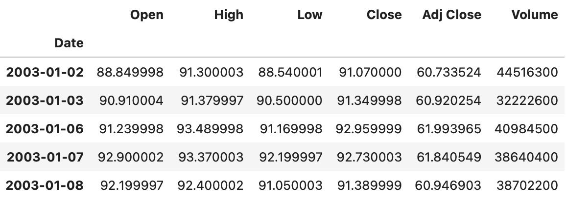
At first we download daily OHLC prices for each instrument. First rows of the resulting dataframe are shown below.
Now we need to resample those dataframes to monthly resolution. In order to calculate each month’s return, we need to have an opening price and a closing price for each month. For closing prices we will use adjusted close prices (as usual), which allow us to account for corporate actions such as dividends, stock splits, etc. Similarly, we need adjusted open prices, but they are not included in our dataset. Therefore I’m going to use a simple trick (described here) to estimate adjusted open prices from adjusted close prices (lines 1-2 in the code below).
| s1_prices['Adj Open'] = s1_prices['Open'] * s1_prices['Adj Close'] / s1_prices['Close'] | |
| s2_prices['Adj Open'] = s2_prices['Open'] * s2_prices['Adj Close'] / s2_prices['Close'] | |
| from collections import OrderedDict | |
| s1_prices_m = s1_prices.resample('1M').agg( | |
| OrderedDict([ | |
| ('Adj Open', 'first'), | |
| ('Adj Close', 'last') | |
| ]) | |
| ) | |
| s2_prices_m = s2_prices.resample('1M').agg( | |
| OrderedDict([ | |
| ('Adj Open', 'first'), | |
| ('Adj Close', 'last') | |
| ]) | |
| ) |
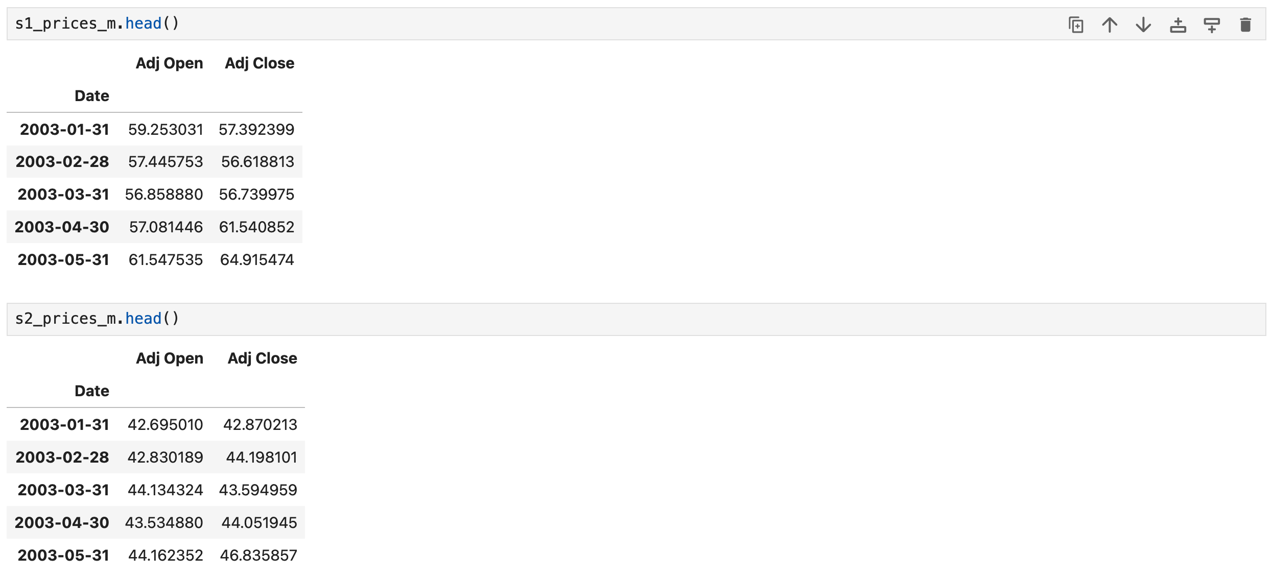
After adjusted open prices are calculated, we resample the data to monthly resolution and obtain the following results.
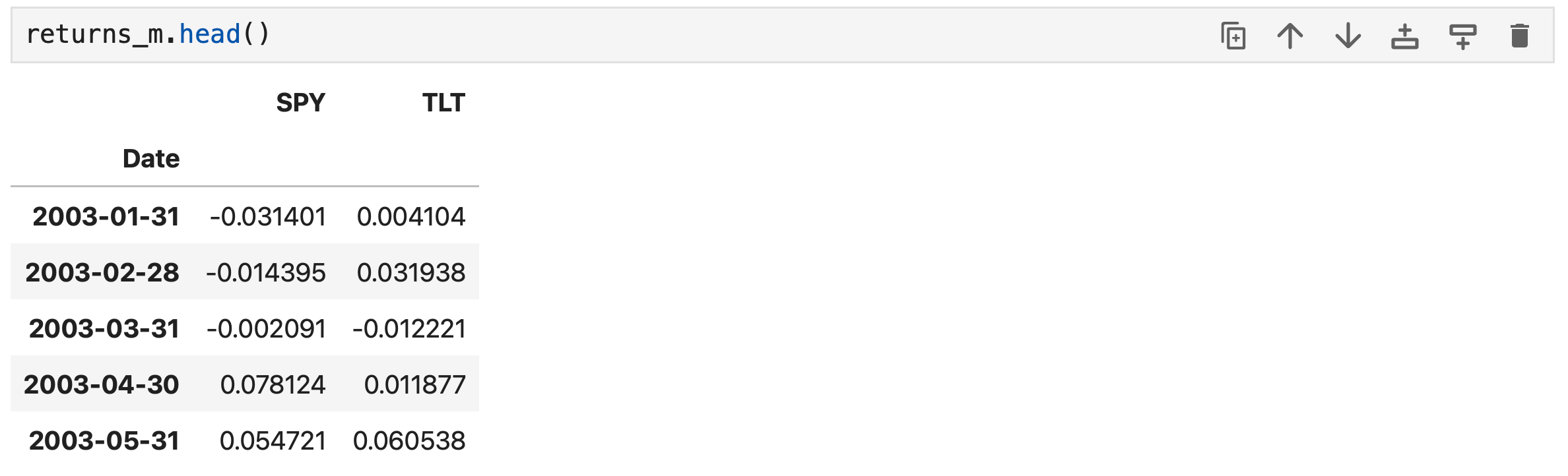
Then we calculate monthly returns of each instrument and combine them in one dataframe.
| returns_m = pd.DataFrame(columns=[s1, s2]) | |
| returns_m[s1] = s1_prices_m['Adj Close'] / s1_prices_m['Adj Open'] - 1 | |
| returns_m[s2] = s2_prices_m['Adj Close'] / s2_prices_m['Adj Open'] - 1 |
The data is prepared and we are ready to implement a backtest.
According to the rules, at the end of each month we need to choose the best performing instrument and invest all our capital in it. As you can see below, this can be done with a few lines of code. Note that I also calculate the cumulative returns of each instrument separately for comparison purposes.
| # prepare positions df | |
| positions = pd.DataFrame(index=returns_m.index, columns=returns_m.columns) | |
| positions[s1] = (returns_m[s1] > returns_m[s2]).astype(int) | |
| positions[s2] = (returns_m[s2] > returns_m[s1]).astype(int) | |
| # calculate return | |
| algo_ret = (positions.shift() * returns_m).sum(axis=1) | |
| # cumulative returns | |
| algo_cumret = (1 + algo_ret).cumprod() | |
| s1_cumret = (1 + returns_m[s1]).cumprod() | |
| s2_cumret = (1 + returns_m[s2]).cumprod() | |
| # make sure that each series start from 1 | |
| algo_cumret /= algo_cumret[0] | |
| s1_cumret /= s1_cumret[0] | |
| s2_cumret /= s2_cumret[0] |
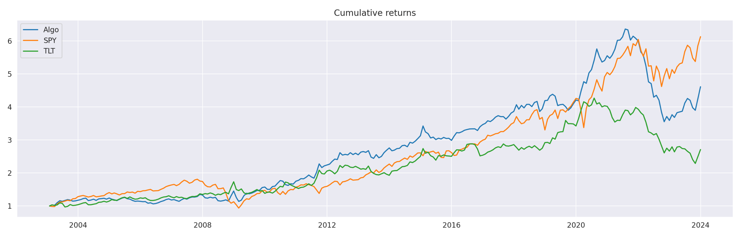
Plot of cumulative returns is shown above. Note that our simple strategy slightly outperforms both SPY and TLT up until some time around 2021. Let’s take a look at the performance metrics.
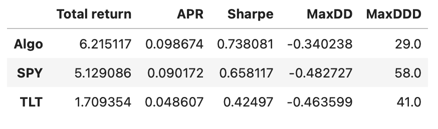
Our algorithm outperforms both individual assets in every calculated metric. Recall that this includes the last few years, where the algorithm didn’t perform very well. Let’s exclude this last part and check how well it performed up until that drop.
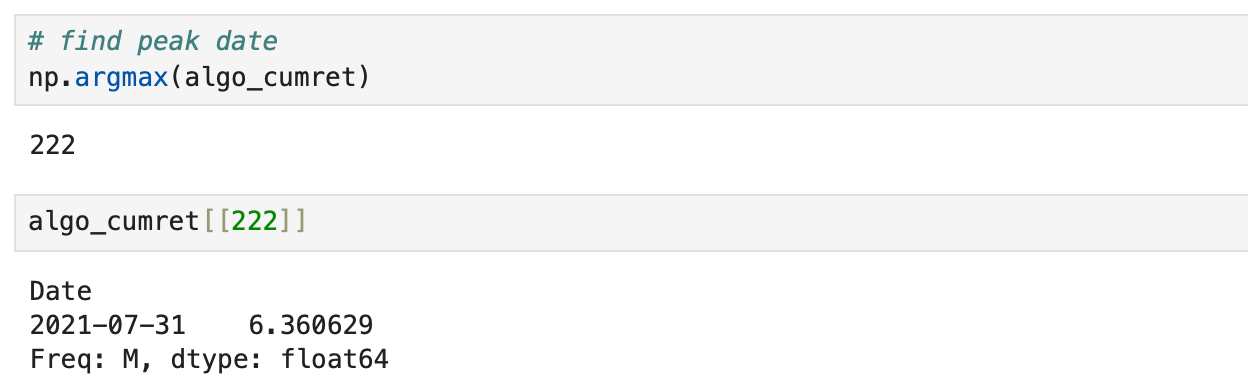
The peak occurred in July 2021, so we will exclude all the data after that point.
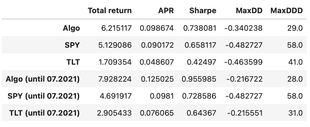
As expected, the algorithm’s performance metrics are even better.
Now let’s try to figure out what makes this simple strategy so profitable. The first thing that comes to mind is our trading signal. Recall that we are simply buying the asset with the best performance during last month. Therefore our signal is the difference between last month’s returns of SPY and TLT. If it is greater than 0, then SPY outperformed TLT during the last month and we expect it to happen again in the following month. If it is lower than zero, then TLT outperformed SPY during the last month and we expect that to repeat. So, basically, our trading signal can be defined as follows:

Let’s calculate and plot it.
| signal = np.sign(returns_m[s1] - returns_m[s2]) | |
| plt.figure(figsize=(18,4)) | |
| plt.plot(signal) | |
| plt.axhline(0, linestyle='dashed', color='r') |
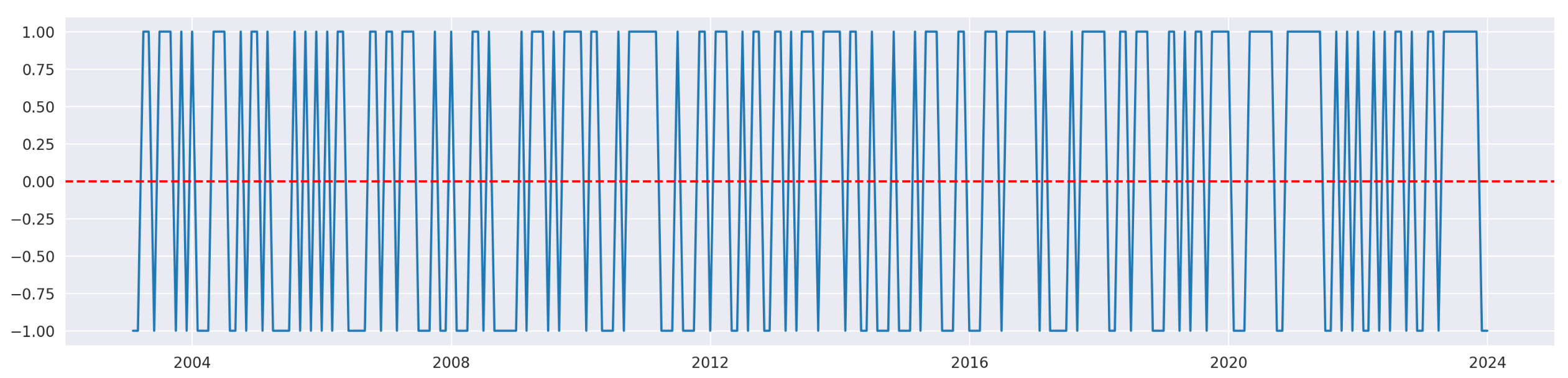
Since we always invest in the asset with the highest return from the previous month, we expect that this same asset will outperform again in the following month. In that case we expect our signal to have a tendency to stay the same. It’s hard to tell from the plot, but it seems that our signal jumps between its two states pretty often.
If the signal tends to stay the same, it should have some autocorrelation. Let’s plot ACF and PACF plots to see if that’s the case.
| import statsmodels.api as sm | |
| fig = plt.figure(figsize=(18,8)) | |
| ax1 = fig.add_subplot(211) | |
| fig = sm.graphics.tsa.plot_acf(signal, ax=ax1) | |
| ax2 = fig.add_subplot(212) | |
| fig = sm.graphics.tsa.plot_pacf(signal, ax=ax2) |
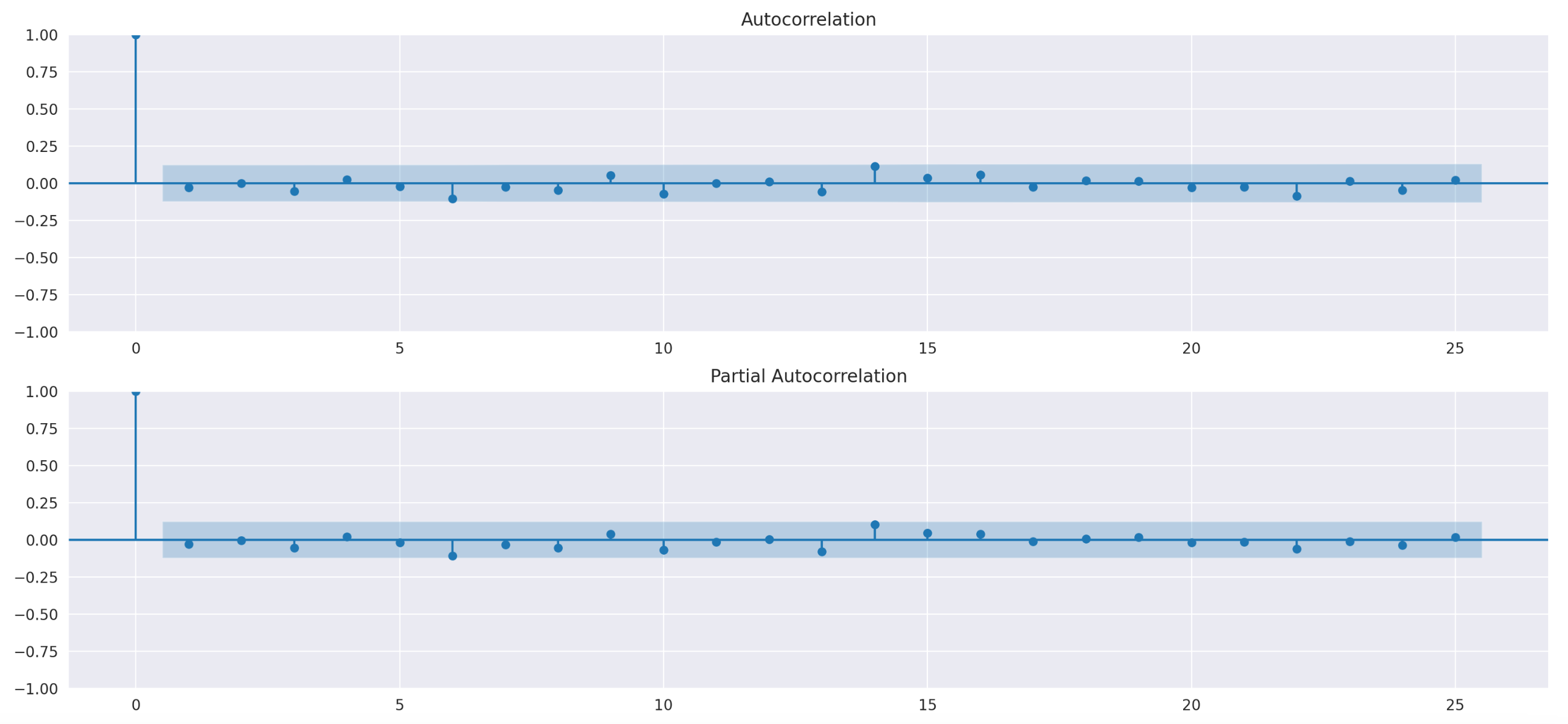
We can’t see any statistically significant autocorrelation in the plots above. Let's calculate how many times it changes from one month to the next, as well as the number and length of periods where it remains unchanged.

It changes on 128 of 252 months and stays the same in 123 of 252 months. This means that our signal is incorrect in 128 of 252 months, giving us a hit rate of 123/252 = 48.8%.
We can try to visually assess the performance of our signal using a confusion matrix.
| from sklearn.metrics import confusion_matrix | |
| # prepare data | |
| y_true = signal.iloc[1:].values | |
| y_pred = signal.shift().iloc[1:].values | |
| # https://www.kaggle.com/code/agungor2/various-confusion-matrix-plots | |
| data = confusion_matrix(y_true, y_pred) | |
| df_cm = pd.DataFrame(data, columns=np.unique(y_true), index = np.unique(y_true)) | |
| df_cm.index.name = 'Actual' | |
| df_cm.columns.name = 'Predicted' | |
| plt.figure(figsize = (4,3)) | |
| sns.heatmap(df_cm, cmap="Blues", annot=True)# font size |
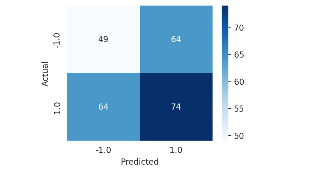
From the plot above, we can see that we have:
49 true negatives,
74 true positives,
64 false negatives,
64 false positives.
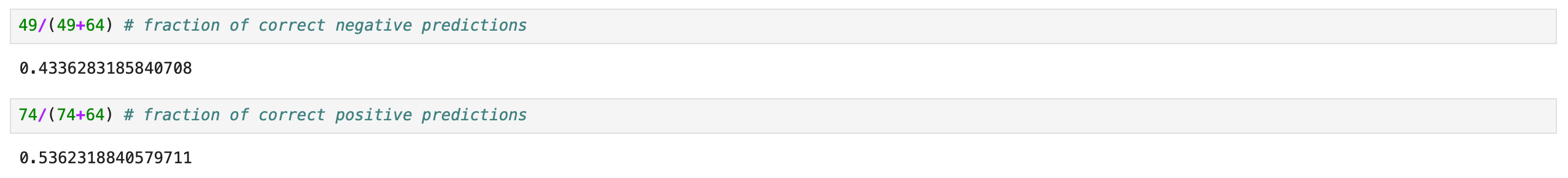
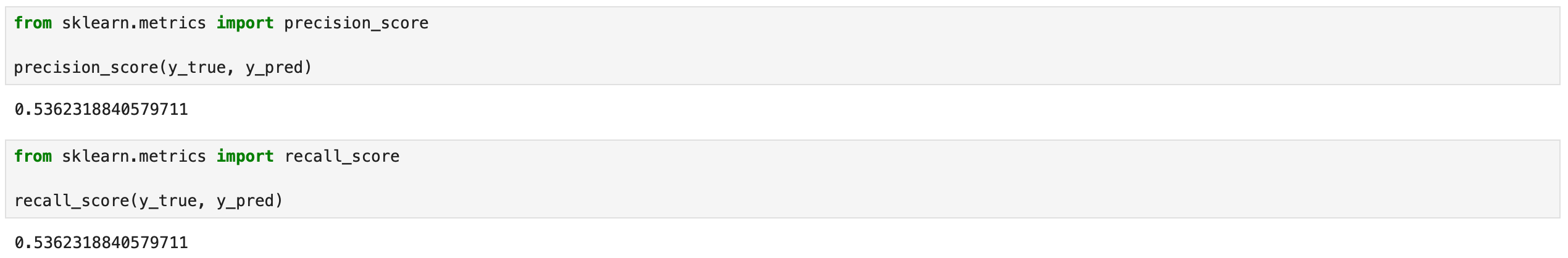
From these numbers, we can calculate a few performance metrics, as shown below.
For comparison take a look at the histograms of precision and recall scores of randomly generated signals.
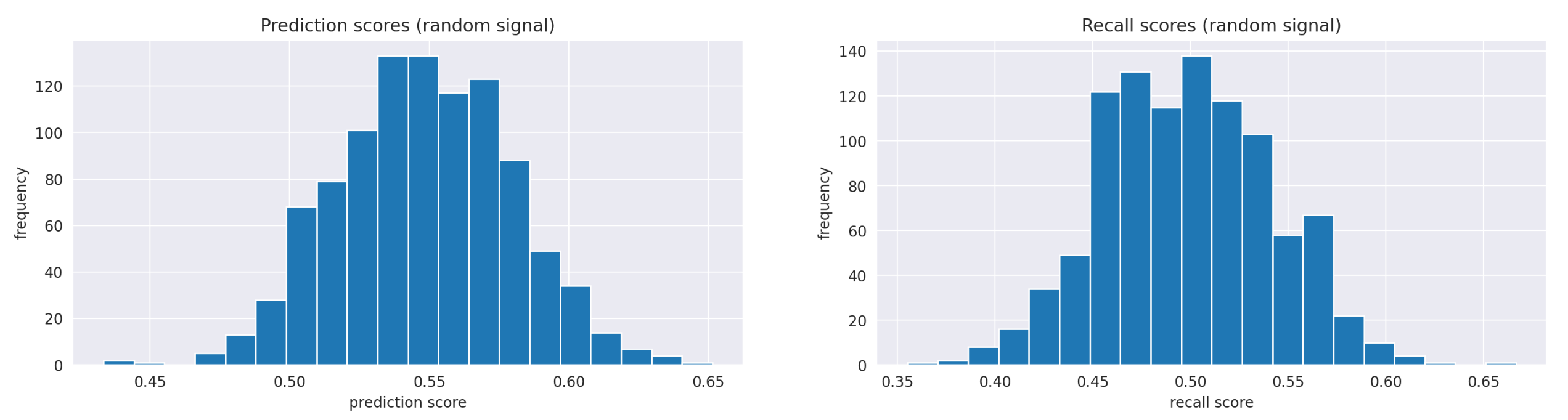
It doesn't look like our signal is performing well. Perhaps the algorithm performs better during larger market movements, helping us avoid significant losses in turbulent markets or capture substantial gains when the market trends. To test this hypothesis, we need to compare the return distributions when the signal's predictions are correct versus when they are incorrect. Let’s split the strategy’s returns into these two groups and calculate their summary statistics.
| ret_signal_correct = algo_ret.iloc[np.where(y_true == y_pred)] # signal's prediction is correct | |
| ret_signal_incorrect = algo_ret.iloc[np.where(y_true != y_pred)] # signal's prediction is incorrect | |
| pd.concat([ret_signal_correct.describe().rename('correct'), ret_signal_incorrect.describe().rename('incorrect')], axis=1) |
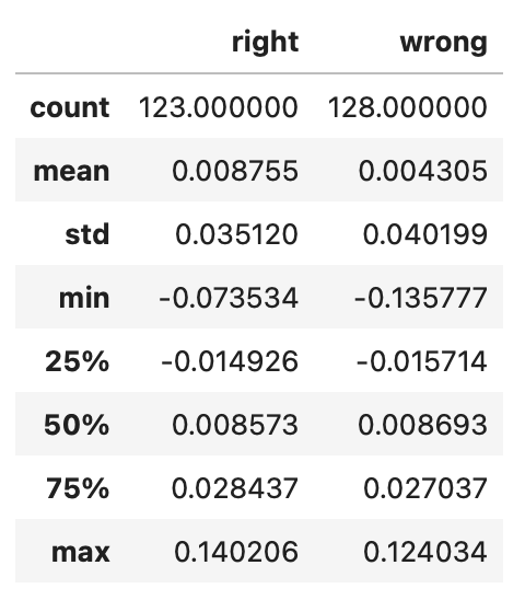
There are some differences in extreme values, but otherwise, both groups look very similar. We can also compare them visually using histograms.
| fig,axs = plt.subplots(1,2,figsize=(18,4)) | |
| axs[0].hist(ret_signal_right, bins=20) | |
| axs[0].set_title('Signal\'s prediction correct') | |
| axs[0].set_xlabel('return') | |
| axs[0].set_ylabel('frequency') | |
| axs[1].hist(ret_signal_wrong, bins=20) | |
| axs[1].set_title('Signal\'s prediction incorrect') | |
| axs[1].set_xlabel('return') | |
| axs[1].set_ylabel('frequency') |
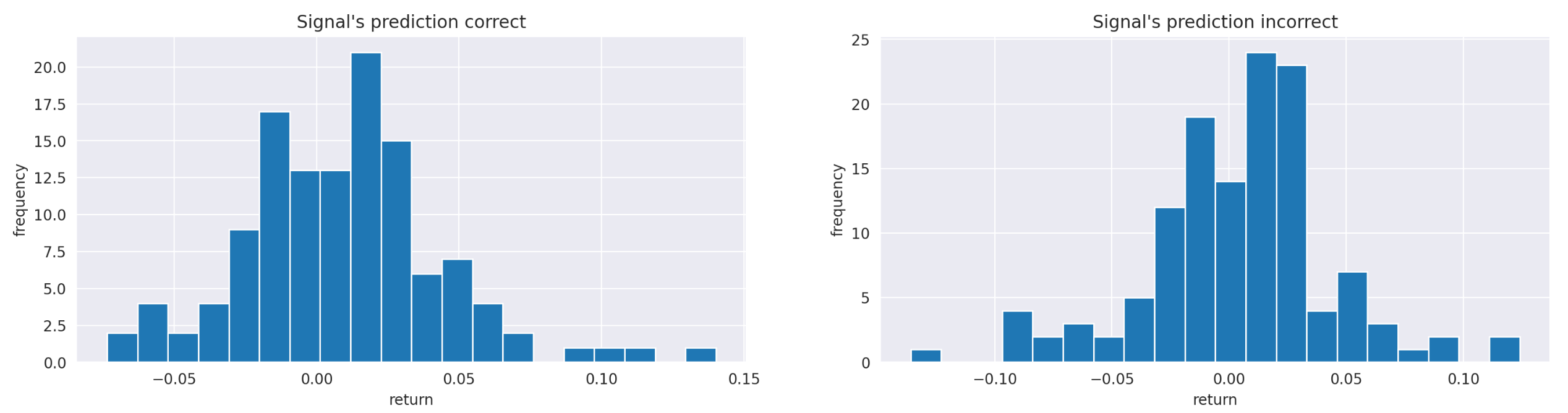
The two histograms look quite similar, so they likely reflect the same underlying distribution. In order to test this hypothesis, we can apply the Kolmogorov-Smirnov test to these two samples.

Recall that the null-hypothesis of Kolmogorov-Smirnov test is that the two samples come from the same distribution. As you can see on the screenshot above, we get a p-value of 0.76. Therefore, we can’t reject the null hypothesis, so we conclude that there is no significant evidence to suggest that the two samples come from different distributions.
So far, we haven’t been able to find any evidence that our signal has any predictive power. Could it be the case that the strategy’s performance is just random? What results will we get if we use random sequences of 1 and -1 as a trading signal? We can easily test that using random simulations. In the code below, I perform 1000 such simulations, saving the performance metrics from each simulation into a dataframe.
| random_signal_metrics = pd.DataFrame(columns=['Total return', 'APR', 'Sharpe', 'MaxDD', 'MaxDDD']) | |
| for i in tqdm(range(1000)): | |
| np.random.seed(i) | |
| signal = np.random.choice([-1,1], size=252) | |
| positions = pd.DataFrame(index=returns_m.index, columns=returns_m.columns) | |
| positions[s1] = (signal>0).astype(int) | |
| positions[s2] = (signal<0).astype(int) | |
| algo_ret = (positions.shift() * returns_m).sum(axis=1) | |
| algo_cumret = (1 + algo_ret).cumprod() | |
| algo_cumret /= algo_cumret[0] | |
| random_signal_metrics.loc[i] = calculate_metrics(algo_cumret) |
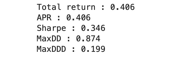
Summary statistics of the resulting dataframe are shown below.
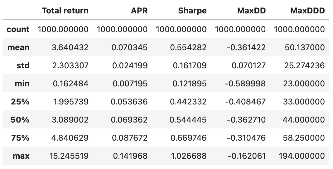
Recall that in our backtest we got the following performance metrics.
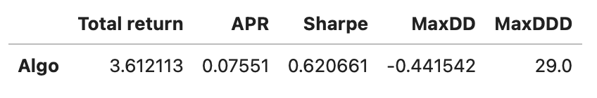
Most metrics are close to the mean values we obtained from random simulations, which means that the performance metrics of the backtest could be driven by randomness. Let’s calculate the fraction of random strategies that outperform our strategy for each metric separately.
| for metric in random_signal_metrics.columns[:-1]: | |
| backtest_val = results_df.loc['Algo'][metric] # value of the metric in backtest | |
| num_outperf = random_signal_metrics[random_signal_metrics[metric]>=backtest_val].shape[0] | |
| print(f'{metric} : {num_outperf / len(random_signal_metrics)}') | |
| # MaxDDD must be LOWER than in backtest | |
| metric = 'MaxDDD' | |
| backtest_val = results_df.loc['Algo'][metric] | |
| num_outperf = random_signal_metrics[random_signal_metrics[metric]<=backtest_val].shape[0] | |
| print(f'{metric} : {num_outperf / len(random_signal_metrics)}') |
As you can see above, a large fraction of random strategies performs better than the strategy we are analyzing. However, here we tested each performance metric individually. Let’s calculate the fraction of random strategies that outperform our strategy across all performance metrics.
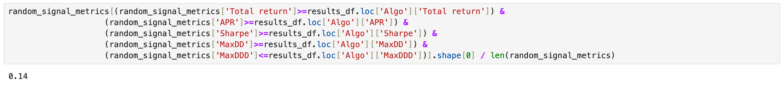
14% of random simulations outperform our strategy in every metric, suggesting that there is a 14% chance our strategy’s performance could be explained by randomness. Furthermore, the trading signal appears random, with no predictive power. Therefore, we can conclude that the backtest results of this strategy are unreliable.
Here are a few ideas that could be used to improve the results:
Trade at a higher frequency (weekly or daily).
Exit the market (sell everything and keep the portfolio in cash) when the returns of both instruments are negative.
Add more assets to trade.
Jupyter notebook with source code is available here.
If you have any questions, suggestions or corrections please post them in the comments. Thanks for reading.
References