Statistical arbitrage with graph clustering algorithms
Applying network theory to statistical arbitrage strategies.

This article is based on the paper ‘Correlation Matrix Clustering for Statistical Arbitrage Portfolios’ (Cartea et al. 2023). The paper describes a framework for constructing statistical arbitrage portfolios using graph clustering algorithms. In this article I will implement and backtest several trading strategies based on the approach described in the paper.
The general algorithm of the strategy is as follows.
Calculate residual returns.
Compute correlation matrix of residuals and interpret it as a weighted signed network.
Use graph clustering algorithms to partition stocks into groups such that, on average, the correlation between stocks in different groups is low, while the correlation within the same group is high.
Employ rolling windows to identify stocks whose returns are above or below the cluster mean.
Construct a contrarian portfolio by taking long positions in ‘losers’ and short positions in ‘winners.'
I will start by implementing different components of the algorithm individually, and then bring them together to create a complete trading strategy.
We begin by preparing the data. I’ll use the same dataset as in my recent articles on portfolio optimization, which includes around 500 assets — constituents of the S&P 500 index. We’ll also need the risk-free rate and market return data to calculate residuals, for which I’ll use data from the Kenneth R. French Data Library. A description of the specific dataset I’m using can be found here.
| prices = pd.read_csv('../sp500.csv', index_col=0) | |
| prices.index = pd.to_datetime(prices.index) | |
| returns = prices.pct_change().iloc[1:] | |
| # factor data | |
| ff_data = pd.read_csv('../F-F_Research_Data_Factors_daily.CSV', skiprows=3, index_col=0).iloc[:-1] | |
| ff_data.index = pd.to_datetime(ff_data.index) | |
| ff_data = ff_data.loc[returns.index] | |
| ff_data /= 100 # percent to decimal |
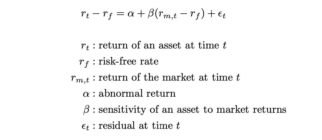
The first step in the algorithm is calculating residuals. We use the following formula to estimate the parameter beta and calculate the residuals epsilon for each asset. Code for this is provided below.
| from sklearn.linear_model import LinearRegression | |
| # estimate betas | |
| returns_rf = returns - ff_data[['RF']].values | |
| res = LinearRegression().fit(ff_data[['Mkt-RF']].values, returns_rf.values) | |
| betas = pd.Series(res.coef_.flatten(), index=returns.columns) | |
| # calculate residuals | |
| resid = pd.DataFrame(index=returns.index, columns=returns.columns) | |
| for s in tqdm(returns.columns): | |
| resid[s] = returns_rf[s] - betas.loc[s] * ff_data['Mkt-RF'] |
To use the clustering algorithms described in the paper, we need to specify the number of clusters. The paper proposes two approaches to estimating this:
RMT (Random Matrix Theory) approach,
Explained variance approach.
Note: In this section I assume that the reader is familiar with the concepts of eigenvalues and eigenvectors in linear algebra; if not, here’s a good introductory video.
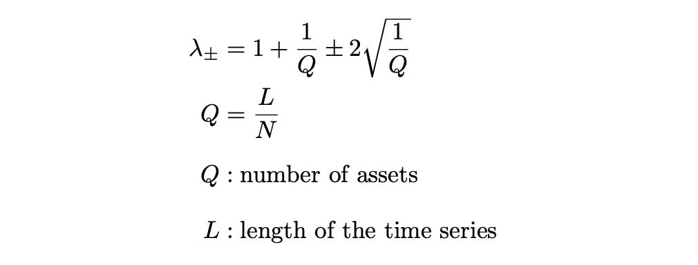
The RMT approach is based on a theorem from Random Matrix Theory, which I discussed in my previous article on portfolio optimization with RMT. Here, the number of clusters equals the number of eigenvalues that exceed a specific threshold, lambda+, which is calculated using the following formulas.
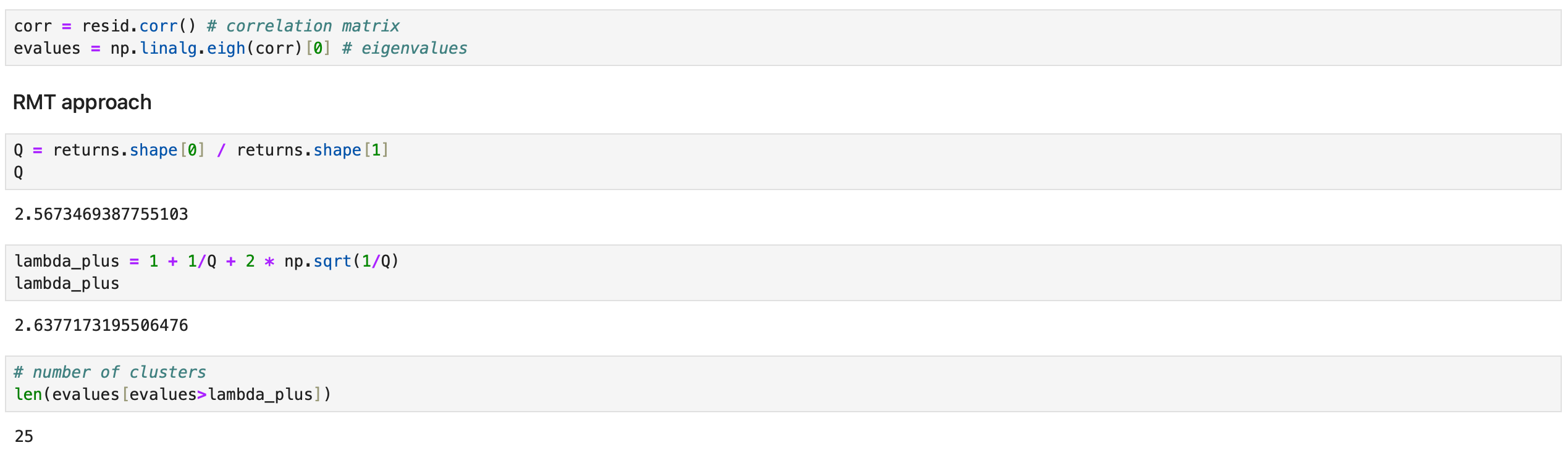
First, we calculate the sample correlation matrix of the residuals and its eigenvalues, then count the number of eigenvalues that exceed the threshold lambda+. The entire procedure is shown on the screenshot below.
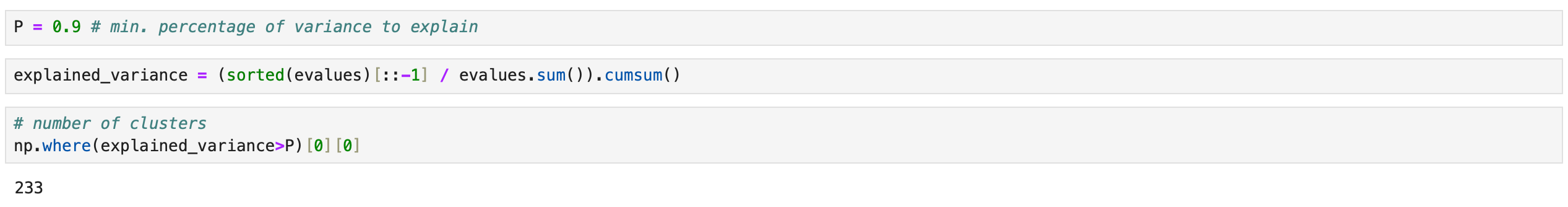
In the explained variance approach, we simply set the number of clusters equal the number of eigenvectors (corresponding to the largest eigenvalues) required to explain a certain percentage of the variance in the data. On the screenshot below, I calculate the number of eigenvectors required to explain 90% of the variability. As you can see, the number obtained here is significantly higher compared to the RMT approach.
Another approach tested in the paper involved manually setting the number of clusters to a fixed value of 30. In this article, I will focus solely on testing the RMT approach.
Now, let’s move on to the final missing piece - the clustering algorithm. Fortunately, all the clustering methods are already implemented in SigNet library, allowing us to use them with just one line of code.
The paper discusses three clustering techniques:
Spectral Clustering.
Signed Laplacian Clustering.
SPONGE (Signed Positive Over Negative Generalised Eigenproblem) clustering.
The pros and cons of these techniques are described in the paper, so I won’t repeat them here. Instead, I’ll simply demonstrate how to use each of them.
The first step for each clustering algorithm is defining a cluster where the correlation matrix is interpreted as an adjacency matrix. The cluster is initialized with separate positive and negative adjacency matrices, both of which must be in Compressed Sparse Column (CSC) format. To convert numpy arrays to CSC, we use the csc_matrix function from the scipy library.
In spectral clustering, we work with the absolute values of the correlation matrix, meaning our negative adjacency matrix will only contain zeros. Defining a cluster and performing clustering is demonstrated below.
| from signet.cluster import Cluster | |
| from scipy.sparse import csc_matrix | |
| c = Cluster((csc_matrix(abs(corr)), csc_matrix(np.zeros(corr.shape)))) | |
| c.spectral_cluster_adjacency(k=25) |
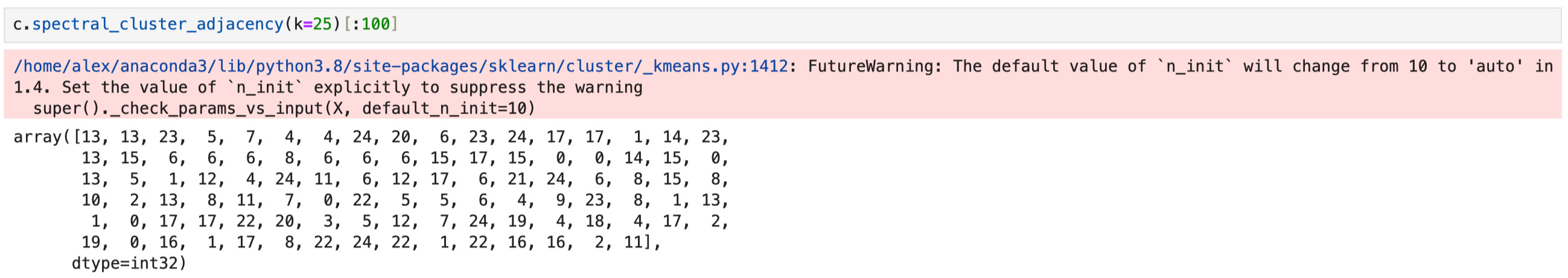
The final result of the clustering is an array of cluster assignments, part of which is shown above.
Now, let’s move on to signed Laplacian clustering. Here, both positive and negative elements are allowed in the adjacency matrix. We split the positive and negative elements of the correlation matrix into separate dataframes, convert them to CSC format, and create a new cluster object. The clustering is performed in the same way, but using a different function.
| # split adjacency matrix into positive and negative | |
| corr_positive = pd.DataFrame(index=corr.index, columns=corr.columns) | |
| corr_negative = pd.DataFrame(index=corr.index, columns=corr.columns) | |
| corr_positive[corr>0] = corr[corr>0] | |
| corr_positive = corr_positive.fillna(0) | |
| corr_negative[corr<0] = -corr[corr<0] | |
| corr_negative = corr_negative.fillna(0) | |
| c = Cluster((csc_matrix(corr_positive), csc_matrix(corr_negative))) | |
| c.spectral_cluster_laplacian(k=25) |
SPONGE clustering uses the same input as Laplacian clustering; it is simply performed with a different function.
| c = Cluster((csc_matrix(corr_positive), csc_matrix(corr_negative))) | |
| c.SPONGE_sym(k=25) |
That’s basically it. We’ve implemented all the key building blocks required to construct a trading strategy.
Now, I will implement and backtest a baseline strategy for comparison purposes. This will be a simple contrarian strategy where, each day, I buy the ‘losers’ (stocks with returns lower than the market) and sell the ‘winners’ (stocks with returns higher than the market). It is similar to the strategies we are going to test, except it only has one cluster.
The code for backtesting is provided below.
| start_date = '2019-01-01' | |
| end_date = '2022-12-31' | |
| # subtract risk-free rate from returns | |
| returns_rf = returns - ff_data[['RF']].values | |
| # calculate positions | |
| positions = pd.DataFrame(index=returns_rf.loc[start_date:end_date].index, columns=returns_rf.columns) | |
| positions[returns_rf < ff_data[['Mkt-RF']].values] = 1 | |
| positions[returns_rf > ff_data[['Mkt-RF']].values] = -1 | |
| # make absolute values of long and short positions sum to 1 | |
| positions[positions>0] *= 1/abs(positions[positions>0].sum(axis=1)).values.reshape(-1,1) | |
| positions[positions<0] *= 1/abs(positions[positions<0].sum(axis=1)).values.reshape(-1,1) | |
| # calculate strategy returns | |
| ret = (positions.shift() * returns.loc[positions.index]).sum(axis=1) | |
| cumret_baseline = (1 + ret).cumprod() |
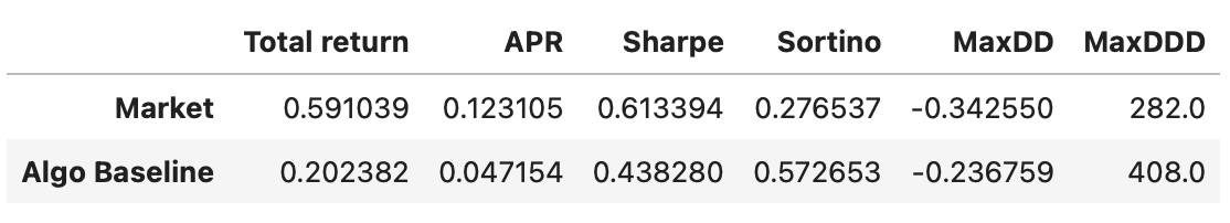
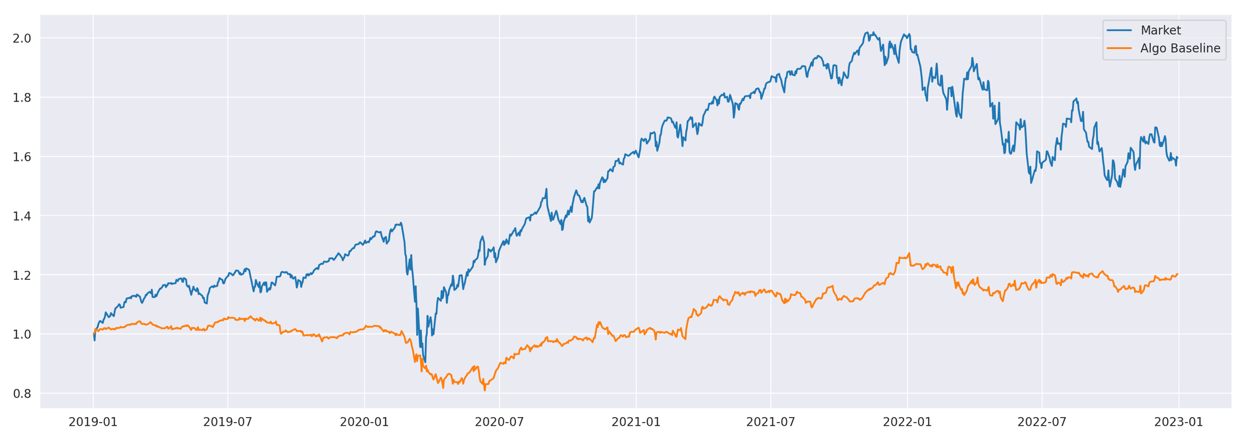
Performance metrics and cumulative returns of the baseline strategy, along with the market, are shown above. Now we are ready to move on to the strategies based on clustering algorithms.
The strategy described in the paper contains many different parameters:
Number of days to estimate the number of clusters: 20
Length of rolling window to estimate beta and compute residuals: 60
Number of lookback days to construct the correlation matrix and compute cluster mean returns: 5
Rebalance period to recompute the correlation matrix, recompute the clusters and rebalance the portfolio: 3
Threshold to identify whether the stock is a winner or a loser: 0
Threshold to consider the portfolio mean reverted (stop-win): 5%
Percentage of winners and losers to select for trading: 100%
Some of the parameters above don’t make sense to me. For example, why use one number of days to estimate the number of clusters and another to estimate beta and compute residuals? Other parameters (like the rebalancing period) are useful in a production environment, but to test whether the trading idea is feasible, we can do without them. Moreover, having a large number of parameters increases the risk of overfitting. Therefore, I’m going to simplify the strategy proposed in the paper and use the following algorithm:
Each day, use a 60-day lookback period to estimate betas, calculate residuals, and compute their sample correlation matrix.
Calculate the eigenvalues of the correlation matrix to estimate the number of clusters and perform clustering.
Calculate the mean returns within each cluster using the same 60-day period and open short positions in winners (assets with returns above the cluster mean) and long positions in losers (assets with returns below the cluster mean).
Ensure that the resulting portfolio is dollar-neutral — the amount of capital allocated to long positions must equal the amount allocated to short positions.
Repeat the process each trading day.
Now the number of parameters has been significantly reduced:
Length of rolling window for historical data: 60
Threshold to identify whether a stock is a winner or a loser: 0
Percentage of winners and losers to select for trading: 100%
Let’s try to backtest it.
Here, I am using a backtesting routine that is slightly different from the one I used in my other articles. I define a function that calculates a row of positions dataframe for each given day. Then, I run this function over the backtesting period and combine the results into a single dataframe. Code for backtesting the strategy using spectral clustering is shown below.
| w = 60 # length of the rolling window | |
| def spectral_clustering_bt(t): | |
| # prepare data | |
| returns_rf_tmp = returns_rf.loc[:t].iloc[-w:] | |
| returns_rf_tmp = returns_rf_tmp.dropna(axis=1) | |
| ff_data_tmp = ff_data.loc[returns_rf_tmp.index] | |
| # compute betas | |
| res = LinearRegression().fit(ff_data_tmp[['Mkt-RF']].values, returns_rf_tmp.values) | |
| betas = pd.Series(res.coef_.flatten(), index=returns_rf_tmp.columns) | |
| # compute residuals | |
| resid = pd.DataFrame(index=returns_rf_tmp.index, columns=returns_rf_tmp.columns) | |
| for s in resid.columns: | |
| resid[s] = returns_rf_tmp[s] - betas.loc[s] * ff_data_tmp['Mkt-RF'] | |
| # estimate the number of clusters | |
| corr = resid.corr() # correlation matrix | |
| evalues = np.linalg.eigh(corr)[0] | |
| Q = returns_rf_tmp.shape[0] / returns_rf_tmp.shape[1] | |
| lambda_plus = 1 + 1/Q + 2*np.sqrt(1/Q) # upper RMT bound | |
| K = len(evalues[evalues>lambda_plus]) # number of clusters | |
| # perform clustering | |
| with warnings.catch_warnings(): | |
| warnings.simplefilter('ignore') | |
| c = Cluster((csc_matrix(abs(corr)), csc_matrix(np.zeros(corr.shape)))) # use absolute values of correlation matrix as input | |
| ca = c.spectral_cluster_adjacency(k=K) | |
| # construct positions | |
| positions = pd.DataFrame(index=[t], columns=returns_rf.columns) | |
| positions = positions.fillna(0) | |
| for cluster in range(K): | |
| c_members = returns_rf_tmp.columns[ca==cluster] | |
| c_winners = returns_rf_tmp[c_members].mean()[returns_rf_tmp[c_members].mean()>returns_rf_tmp[c_members].mean().mean()].index | |
| c_losers = returns_rf_tmp[c_members].mean()[returns_rf_tmp[c_members].mean()<returns_rf_tmp[c_members].mean().mean()].index | |
| positions.loc[t, c_winners] = -1 / len(c_winners) # short position in winners | |
| positions.loc[t, c_losers] = 1 / len(c_losers) # long_position in losers | |
| return positions | |
| positions = pd.concat([spectral_clustering_bt(t) for t in returns_rf.loc[start_date:end_date].index]) | |
| # make absolute values of long and short positions sum to 1 | |
| positions[positions>0] *= 1/abs(positions[positions>0].sum(axis=1)).values.reshape(-1,1) | |
| positions[positions<0] *= 1/abs(positions[positions<0].sum(axis=1)).values.reshape(-1,1) | |
| # calculate strategy returns | |
| ret = (positions.shift() * returns.loc[positions.index]).sum(axis=1) | |
| cumret_spectral = (1 + ret).cumprod() |
The other strategies are similar; only the clustering part changes. I won’t post their code here, but you can find it in the corresponding Jupyter notebook.
Let’s take a look at final results. Performance metrics and cumulative returns of each strategy are shown below. Note that, due to the randomness involved in clustering algorithms, your results might vary slightly.
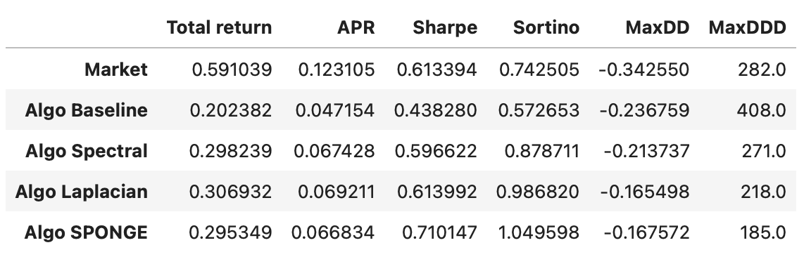
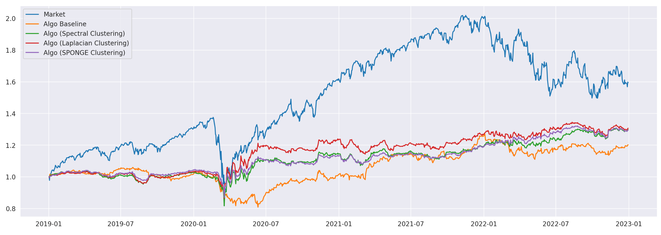
In terms of Sharpe ratios, all algorithms are approximately the same. However, if we look at their Sortino ratios, the strategies based on Laplacian and SPONGE clustering algorithms significantly outperform the other strategies and the overall market. Although the total return of these strategies is lower than the market, the strategies are dollar-neutral, allowing us to use leverage to increase returns without changing the underlying risk-adjusted performance (Sharpe and Sortino ratios).
Ideas for further research:
Try using other factor models for calculating residuals.
Adjust the lengths of lookback windows and introduce stop-wins and stop-losses, as described in the paper.
Test different approaches to estimating the number of clusters.
Perform some analysis of the clusters computed by each clustering algorithm.
In conclusion, we have explored the use of graph clustering algorithms to construct statistical arbitrage strategies. While all strategies showed similar Sharpe ratios, clustering-based approaches stood out in terms of Sortino ratios, indicating better downside risk management.
This study demonstrates the potential of clustering-based approaches in statistical arbitrage and emphasizes the importance of further research to refine and optimize these methods for practical trading scenarios.
Jupyter notebook with source code is available here.
If you have any questions, suggestions or corrections please post them in the comments. Thanks for reading.
References
[1] Correlation Matrix Clustering for Statistical Arbitrage Portfolios (Cartea et al. 2023)
[2] SigNet - a package for clustering of signed networks
[3] Portfolio Optimization. Random Matrix Approach to Estimating Covariance Matrix