

Statistical arbitrage with lead-lag detection
Revealing market leaders and followers through linear and non-linear relationships.

This article is based on the paper ‘Detecting Lead-Lag Relationships in Stock Returns and Portfolio Strategies’ (Cartea et al. 2023). It proposes a few different metrics to detect lead-lag relationships in asset returns and rank assets from leaders to followers. In one of my previous articles I described using Granger causality test for uncovering lead-lag relationships in pairs trading. But that test is only able to detect linear relationships. One of the metrics proposed in the paper is able to detect non-linear relationships.
First let’s try to understand the metrics for identifying pairwise lead-lag relationships provided in the paper. I believe I’ve found a couple of mistakes in the provided formulas and I’m going to explain them here. If you think I’m mistaken, please share your thoughts in the comments.
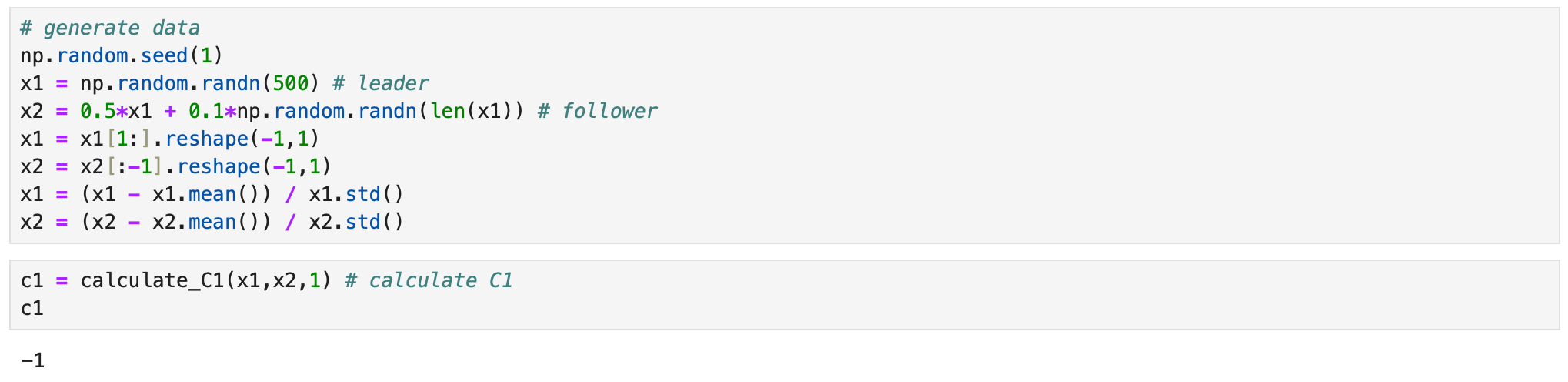
The formula for calculating C1 metric from the paper is shown below.

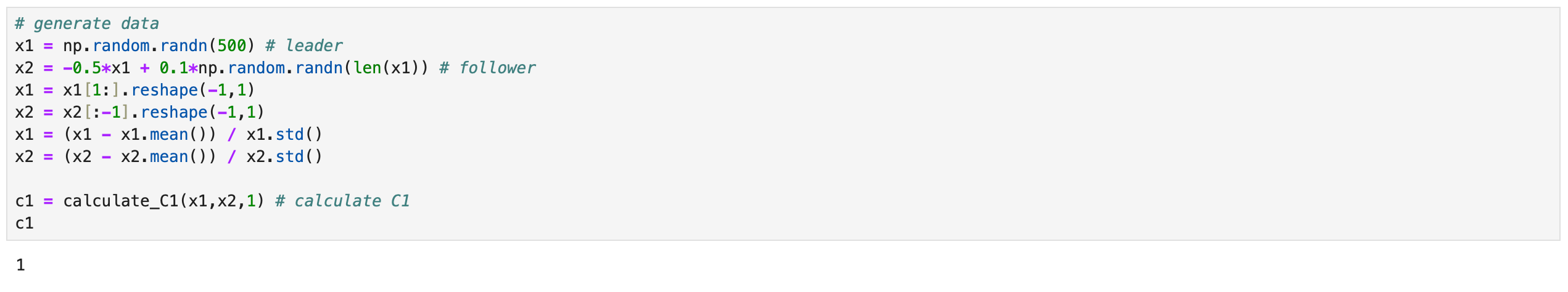
According to the text, we expect its value to be large when asset p leads asset q. But suppose l=T. Then we are calculating the correlation between the returns of asset p with lagged (by T) returns of asset q. If this correlation is large, it indicates that asset p is a follower, not a leader. But according to the formula, C1 metric will be high, indicating that p is a leader. This is demonstrated in the example below.
| def lagged_corr(x1,x2,l): | |
| ''' | |
| compute correlation between x1_{t} and x2_{t-l} | |
| x1 : array_like (n_obs * 1) | |
| x2 : array_like (n_obs * 1) | |
| l : int | |
| ''' | |
| if l>0: | |
| corr = np.corrcoef(x1[l:].T,x2[:-l].T)[0][1] # l positive -> x1 is a follower | |
| elif l==0: | |
| corr = np.corrcoef(x1.T,x2.T)[0][1] | |
| elif l<0: | |
| corr = np.corrcoef(x1[:l].T,x2[-l:].T)[0][1] # l negative -> x2 is a follower | |
| return corr | |
| def calculate_C1(x1,x2,T): | |
| ''' | |
| calculate C1 score between x1 and x2 for maxlag T | |
| x1 : array_like (n_obs * 1) | |
| x2 : array_like (n_obs * 1) | |
| T : int | |
| ''' | |
| correlations = {l:lagged_corr(x1,x2,l) for l in range(-T,T+1)} | |
| return max(correlations, key=correlations.get) |
To fix this issue we just need to change the sign in front of l from - to +, resulting in the following formula.

To fix it in code we just need to update the function for calculating lagged correlations as follows.
| def lagged_corr(x1,x2,l): | |
| ''' | |
| compute correlation between x1_{t} and x2_{t-l} | |
| x1 : array_like (n_obs * 1) | |
| x2 : array_like (n_obs * 1) | |
| l : int | |
| ''' | |
| if l>0: | |
| corr = np.corrcoef(x1[:-l].T,x2[l:].T)[0][1] | |
| elif l==0: | |
| corr = np.corrcoef(x1.T,x2.T)[0][1] | |
| elif l<0: | |
| corr = np.corrcoef(x1[-l:].T,x2[:l].T)[0][1] | |
| return corr |
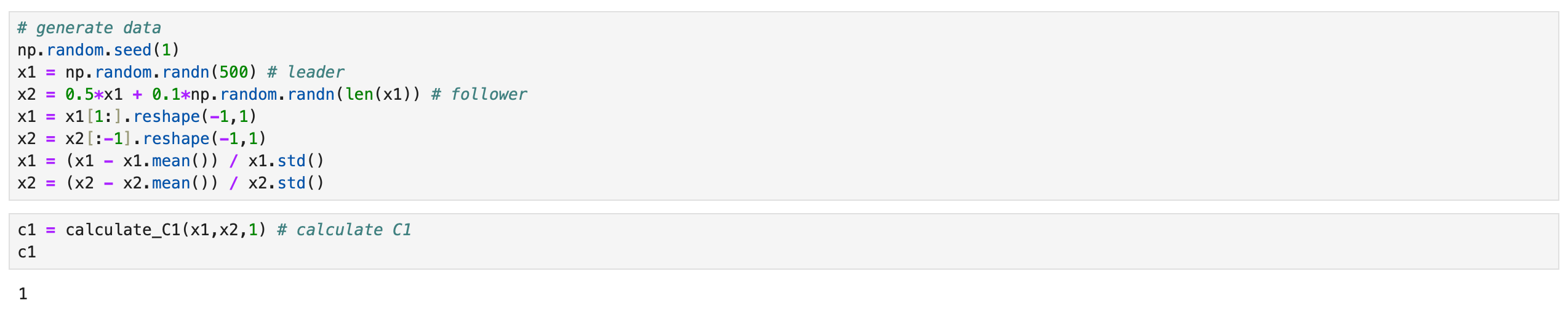
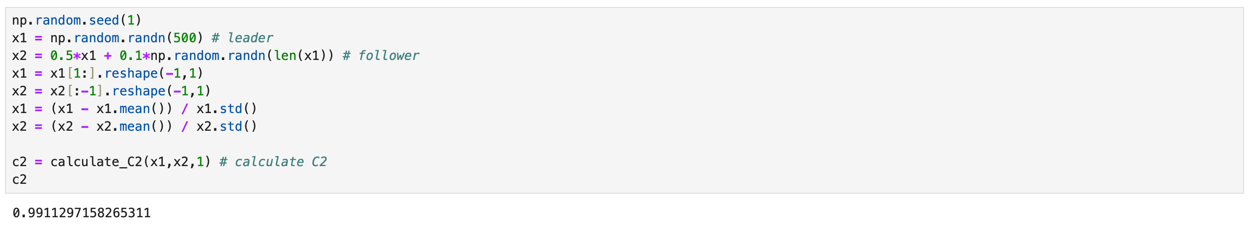
As you can see above, now we get the correct result from the same data. But let’s take a look at another example.
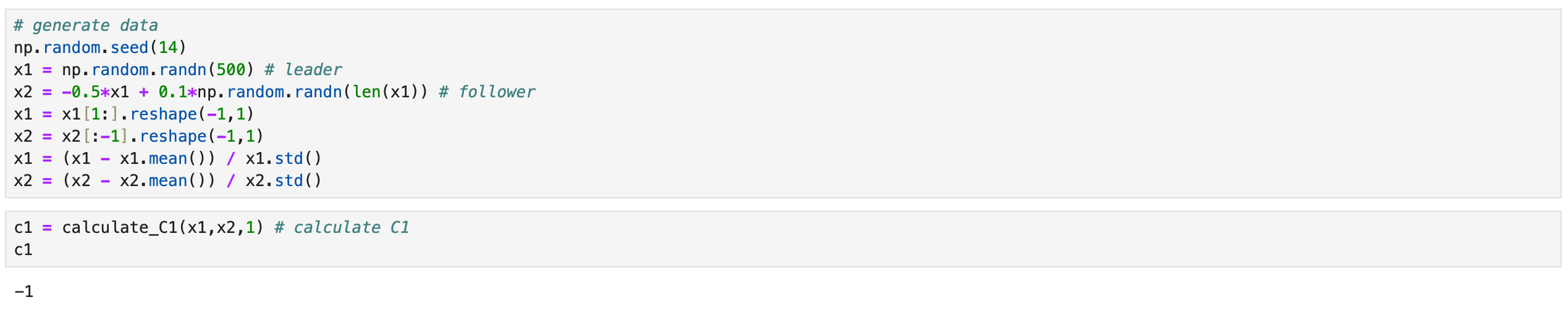
Everything is basically the same, I only change the sign of the x1 coefficient in x2, so that now they are negatively correlated. x1 is still a leader, but according to the metric, it is not.

Taking a look at lagged correlations we can quickly understand the issue - our formula doesn’t take into account that negative value of correlation coefficient can also mean high correlation. Updated formula is provided below. Now we are calculating the absolute values of the correlations.

To update it in code, we just need to update the calculate_C1 function as shown below.
| def calculate_C1(x1,x2,T): | |
| ''' | |
| calculate C1 score between x1 and x2 for maxlag T | |
| x1 : array_like (n_obs * 1) | |
| x2 : array_like (n_obs * 1) | |
| T : int | |
| ''' | |
| correlations = {l:abs(lagged_corr(x1,x2,l)) for l in range(-T,T+1)} | |
| return max(correlations, key=correlations.get) |
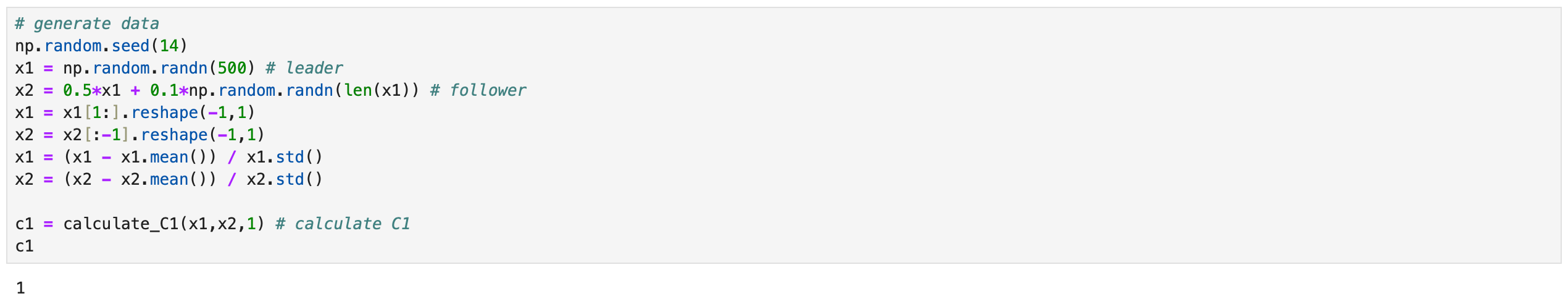
Repeating the previous examples we now get correct results. It seems that the C1 metric works fine now (at least I wasn’t able to find any other issues).
Now let’s try to implement the C2 metric. Formula from the paper is shown below.

Here again we should use absolute values of correlations in order to take into account the cases where the assets are negatively correlated. The sign in front of l is not important here, but I’m going to change it anyway for consistency with the first metric.

The sign of the metric changes, depending on which sum is bigger:
when the first sum is bigger, then asset p is a follower and the metric must be negative,
when the second sum is bigger, then asset p is a leader and the metric must be positive.
Code for calculating the metric is provided below.
| def calculate_C2(x1,x2,T): | |
| ''' | |
| calculate C2 score between x1 and x2 for maxlag T | |
| x1 : array_like (n_obs * 1) | |
| x2 : array_like (n_obs * 1) | |
| T : int | |
| ''' | |
| corr_nlag = [] # correlations for negative lags | |
| for l in range(-T,1): | |
| corr = lagged_corr(x1,x2,l) | |
| corr_nlag.append(corr) | |
| corr_plag = [] # correlations for negative lags | |
| for l in range(0,T+1): | |
| corr = lagged_corr(x1,x2,l) | |
| corr_plag.append(corr) | |
| sum1 = np.abs(corr_nlag).sum() | |
| sum2 = np.abs(corr_plag).sum() | |
| if sum1>sum2: | |
| c2 = -1/T * sum1 | |
| elif sum2>sum1: | |
| c2 = 1/T * sum2 | |
| return c2 |
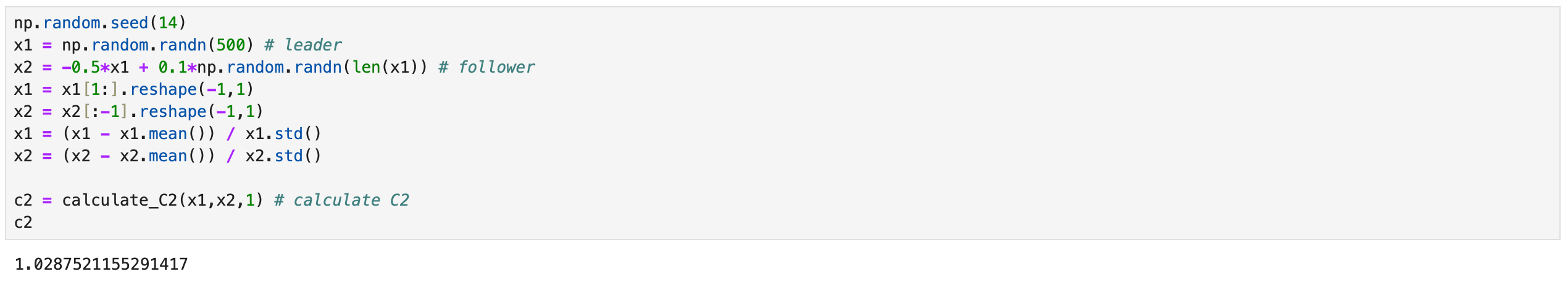
On the screenshots below I repeat the same examples I used for the first metric to make sure that we get the correct results.
The third metric is the most interesting one. It is based on the concept of Levy area, which allows to detect non-linear lead-lag relationships between the time series. I’m not familiar with the theory behind this concept, but luckily there is a python library, where it is implemented. There is a small tutorial on the library’s GitHub page, where you can learn more about rough path theory, signatures and Levy area.
To calculate Levy area between two time series, we need to calculate the signatures first, as demonstrated below.
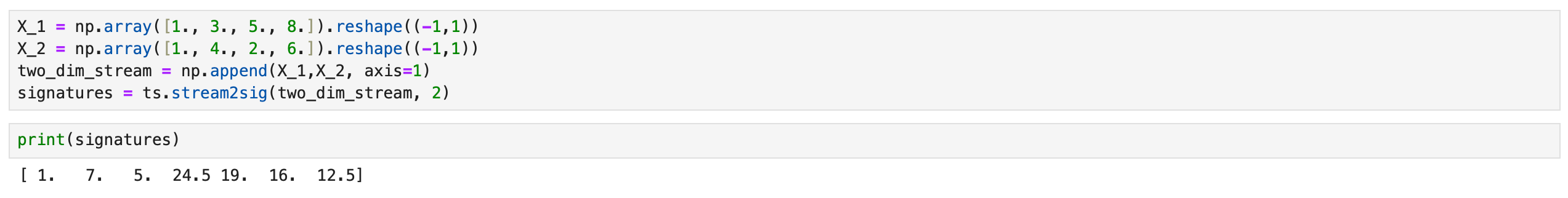
The signatures are returned in the following order.

Now we can calculate Levy area using the formula provided below.


Now I am going to repeat the Monte Carlo simulation, described in the paper, to assess the performance of different metrics. Code for it is shown below.
| levy_areas = [] | |
| C1s = [] | |
| C2s = [] | |
| for i in tqdm(range(50000)): | |
| # generate data | |
| np.random.seed(i) | |
| x1 = np.random.randn(500) # leader | |
| x2 = 10/(1 + np.exp(-x1)) + 5/(1 + np.exp(10*x1)) - 7.5 # follower | |
| x1 = x1[1:].reshape(-1,1) | |
| x2 = x2[:-1].reshape(-1,1) | |
| x1 = (x1 - x1.mean()) / x1.std() # standardize x1 | |
| x2 = (x2 - x2.mean()) / x2.std() # standardize x2 | |
| two_dim = np.append(x1,x2,axis=1) # combine in one array | |
| signatures = ts.stream2sig(two_dim,2) # compute signatures | |
| A_12 = 1/2 * (signatures[4] - signatures[5]) # calculate Levy area | |
| c1 = calculate_C1(x1,x2,1) # calculate C1 | |
| c2 = calculate_C2(x1,x2,1) # calculate C2 | |
| # save results | |
| levy_areas.append(A_12) | |
| C1s.append(c1) | |
| C2s.append(c2) | |
| levy_areas = np.array(levy_areas) | |
| C1s = np.array(C1s) | |
| C2s = np.array(C2s) |
Now we calculate the percentage of simulations where a given metric correctly identifies the leader.
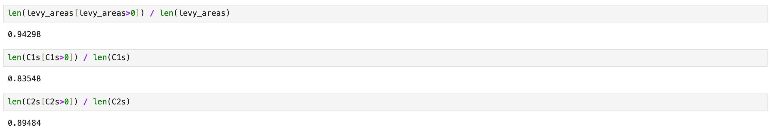
The numbers are a little different from the paper, but Levy area still has the best performance.
Now we are ready to implement and backtest a trading strategy based on those metrics. It works as follows:
At the end of each trading period we calculate the chosen metric for each asset to identify assets-leaders and assets-followers. I’m doing it daily using 60-day lookback window.
Sort the assets based on a calculated metric from most likely to be a leader to most likely to be a follower and select top 20% as leaders and bottom 20% as followers.
If the leaders have positive mean return during the last trading period (last day), we expect the followers to have positive mean return at the next trading period. Therefore we open long position in followers and short the market to finance that position.
If the leaders have negative mean returns, we open a short position in followers and long position in the market.
Rebalance portfolio daily.
I will show the code for backtesting a strategy based on C1 metric here, the rest you can find in the corresponding Jupyter notebook. First I define parameters of the strategy as shown on the screenshot below.

Then I create a function to calculate a line of positions dataframe for a given day. That function is then executed with ProcessPoolExecutor class in order to utilise all processors in parallel.
| def backtest_c1(t): | |
| # prepare data | |
| returns_tmp = returns.loc[:t].iloc[-w:].dropna(axis=1) | |
| returns_tmp = returns_tmp.drop('Mkt', axis=1) # remove market returns | |
| # construct matrix C | |
| c1_matrix = pd.DataFrame(index=returns_tmp.columns, columns=returns_tmp.columns) | |
| for s1 in c1_matrix.index: | |
| for s2 in c1_matrix.columns: | |
| if s1!=s2 and np.isnan(c1_matrix.loc[s1][s2]): | |
| c1 = calculate_C1(returns_tmp[s1].values, returns_tmp[s2].values, maxlag) | |
| c1_matrix.loc[s1][s2] = c1 | |
| c1_matrix.loc[s2][s1] = -c1 | |
| c1_matrix = c1_matrix.astype(float) | |
| # define leaders and followers | |
| leaders = c1_matrix.mean(axis=1).sort_values().iloc[-num_leaders:].index | |
| followers = c1_matrix.mean(axis=1).sort_values().iloc[:num_followers].index | |
| # construct positions dataframe | |
| positions = pd.DataFrame(index=returns_tmp.iloc[-1:].index, columns=returns.columns) | |
| if returns_tmp.loc[t][leaders].mean()>=0: | |
| positions.loc[t, followers] = 1 # long position in followers | |
| positions.loc[t, ['Mkt']] = -len(followers) # short position in the market | |
| else: | |
| positions.loc[t, followers] = -1 # short position in followers | |
| positions.loc[t, ['Mkt']] = len(followers) # long position in the market | |
| return positions, c1_matrix |
| from concurrent.futures import ProcessPoolExecutor | |
| e = ProcessPoolExecutor() | |
| futures = [e.submit(backtest_c1, t) for t in prices.iloc[w:].index] | |
| positions = pd.concat([f.result()[0] for f in futures]) | |
| # make absolute values of long and short positions sum to 1 | |
| positions[positions>0] *= 1/abs(positions[positions>0].sum(axis=1)).values.reshape(-1,1) | |
| positions[positions<0] *= 1/abs(positions[positions<0].sum(axis=1)).values.reshape(-1,1) | |
| # calculate strategy returns | |
| ret = (positions.shift() * returns.loc[positions.index]).sum(axis=1) | |
| cumret_c1 = (1 + ret).cumprod() | |
| # calculate market cumulative return | |
| cumret_market = (1 + returns.loc[positions.index, 'Mkt']).cumprod() | |
| results_df = pd.DataFrame(columns=['Total return', 'APR', 'Sharpe', 'Sortino', 'MaxDD', 'MaxDDD']) | |
| results_df.loc['Market'] = calculate_metrics(cumret_market) | |
| results_df.loc['Algo C1'] = calculate_metrics(cumret_c1) |
Other strategies are similar. I just update the function to use different lead-lag metric. Everything else is the same. Performance metrics of all the strategies are shown below.
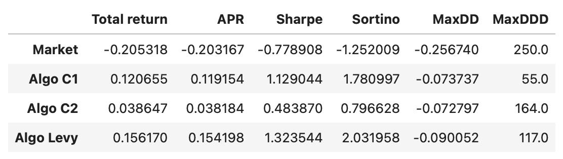
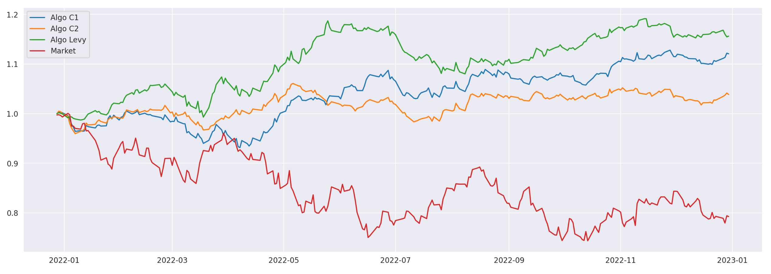
As you can see, all of the strategies outperform the market, which was down 20% in the tested period. The strategy based on Levy area has the best performance in terms of APR and Sharpe\Sortino ratios. Its drawdown is a little larger and longer than that of C1 strategy, but still not bad. Let’s also take a look at the cumulative returns of the algorithms.
I believe that the strategy is interesting and deserves further exploration. One of the ideas for further improvement, proposed in the paper, is using clustering algorithms (described in my previous article) to first split assets into clusters and then identify leaders and followers within each cluster.
Jupyter notebook with source code is available here.
If you have any questions, suggestions or corrections please post them in the comments. Thanks for reading.
References
[1] Detecting Lead-Lag Relationships in Stock Returns and Portfolio Strategies (Cartea et al. 2023)
Great job! Love your work!